
ChemicaLite 是一个基于 RDKit 的 SQLite 数据库扩展,专为化学信息学应用设计。可在化合物库中搜索目标分子,支持子结构搜索和相似性搜索两种模式。
核心特性:
适用场景:
查询分子文件,支持多个文件,格式为 .sdf、.smi、.smiles
私有化合物库文件路径,与 Public Library 二选一
搜索方法,可选值:
sim相似性阈值,范围 0.0-1.0,默认为 0.7,仅在相似性搜索时有效
输出 SDF 文件路径,默认为 hits.sdf
命中信息 CSV 文件路径,默认为 hits.csv
输出结果包括:
| 文件名 | 说明 |
|---|---|
hits.sdf |
命中分子的 SDF 文件 |
hits.csv |
命中信息 CSV 文件(可选) |
其中 SDF 文件包含以下分子属性:
| 属性名 | 说明 |
|---|---|
QUERY_NAME |
查询分子名称 |
QUERY_FILE |
查询文件路径 |
QUERY_INDEX |
查询分子序号 |
SEARCH_METHOD |
搜索方法 |
HIT_INDEX |
命中序号 |
HIT_ID |
命中分子 ID |
SIMILARITY |
相似性分数(仅相似性搜索) |
其中 hits.csv 包含信息如下:
| 列名 | 说明 |
|---|---|
query_name |
查询分子名称 |
query_file |
查询文件路径 |
query_index |
查询分子序号 |
hit_id |
命中分子 ID |
similarity |
相似性分数 |
ChemicaLite is a SQLite database extension built on RDKit, designed for cheminformatics applications. It enables searching for target molecules within compound libraries, supporting two modes: substructure search and similarity search.
Key features:
rdtree indexingUse cases:
Query molecule file(s); multiple files supported. Accepted formats: .sdf, .smi, .smiles.
Path to a private compound library file. Mutually exclusive with Public Library.
Search algorithm. Options:
sim — Similarity search based on Tanimoto coefficientsub — Substructure search based on SMARTS matchingsimSimilarity threshold in the range 0.0–1.0. Default: 0.7. Applies to similarity search only.
Output SDF file path. Default: hits.sdf.
Output CSV file path for hit information. Default: hits.csv.
Results consist of two files:
| File | Description |
|---|---|
hits.sdf |
SDF file containing hit molecules |
hits.csv |
CSV file with hit metadata (optional) |
SDF molecule properties:
| Property | Description |
|---|---|
QUERY_NAME |
Query molecule name |
QUERY_FILE |
Query file path |
QUERY_INDEX |
Query molecule index |
SEARCH_METHOD |
Search method used |
HIT_INDEX |
Hit index |
HIT_ID |
Hit molecule ID |
SIMILARITY |
Similarity score (similarity search only) |
hits.csv columns:
| Column | Description |
|---|---|
query_name |
Query molecule name |
query_file |
Query file path |
query_index |
Query molecule index |
hit_id |
Hit molecule ID |
similarity |
Similarity score |

PepCraft 是唯信开发的从头多肽生成模型,用于面向蛋白受体热点区域设计候选结合多肽。
用户提供受体序列、目标 hotspot、多肽长度和多肽类型后,PepCraft会生成多肽候选,并使用 Boltz-2 对受体-多肽复合物进行结构预测与打分,最终输出按综合评分排序的设计结果。
当前支持三种多肽类型:

相比于EvoBind等多肽设计方法,PepCraft在生成的质量和多样性方面具有显著优势,同时支持线性、环肽等各种多肽类型。
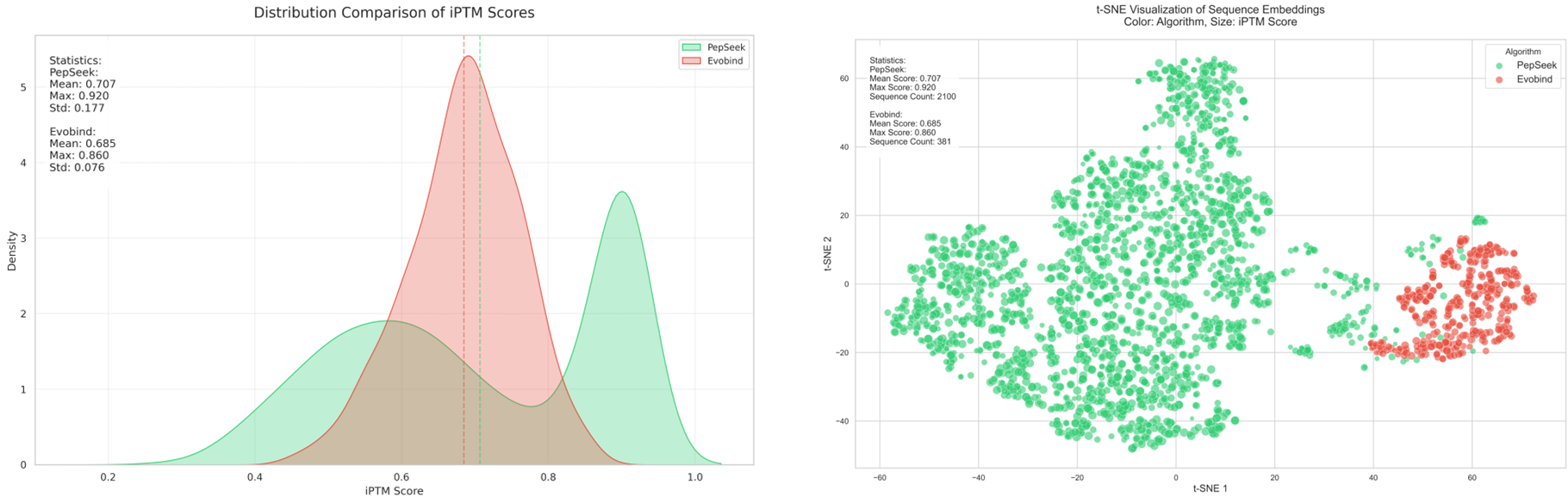
注:上图中PepSeek即为PepCraft
PepCraft 的核心流程为“候选生成 - 结构验证 - 指标评分 - 迭代优化”。候选多肽可由 PepMLM、随机生成、突变和交叉等方式产生;结构验证阶段使用 Boltz-2 预测复合物,并结合整体置信度、界面质量和 hotspot 接触情况进行综合排序。
为提升运行效率,流程会在每次任务开始时仅对受体序列搜索一次 MSA,后续所有候选多肽验证时复用该受体 MSA;多肽链始终使用 single-sequence mode,不单独搜索 MSA。
受体蛋白序列文件。支持标准 FASTA 单行序列、标准 FASTA 多行序列,以及无 header 的纯序列输入。
流程会自动进行格式检查与标准化,包括:
示例:
>1SSC_1|Chain A|RIBONUCLEASE A
KETAAAKFERQHMDSSTSAASSSNYCNQMMKSRNLTKDRCKPVNTFVHESLADVQAVCSQKNVACKNGQTNCYQSYSTMSITDCRETGSSKYPNCAYKTTQANKHIIVACEG
受体上的目标结合热点残基,使用 1-indexed 编号。支持单个残基、多个残基和连续区间。
示例:
15,16
20-24,31
目标多肽长度。
示例:
15
多肽的化学类型或结构约束,用于限定生成多肽的理化性质,可选参数。
linear:线性多肽,无环化约束disulfidecyclic:环化多肽,首尾或侧链形成环化结构其中 disulfide 会约束多肽首尾为半胱氨酸,并在结构预测输入中加入首尾二硫键约束;cyclic 会在结构预测输入中设置环肽约束。
PepCraft 输出打包结果 results.zip,其中包含按综合评分排序的候选多肽信息和对应结构文件。
主要输出文件包括:
| 文件 | 含义 |
|---|---|
top_designs.csv |
Top 设计结果汇总表,默认输出前 20 个候选。 |
rank_1.cif, rank_2.cif, … |
按评分排序后的受体-多肽复合物结构文件。 |
results.zip |
最终交付压缩包,包含 top_designs.csv 和 ranked CIF 文件。 |
top_designs.csv 输出以下信息:
| 列名 | 含义 |
|---|---|
rank |
设计结果排名,按综合评分排序。 |
design_id |
设计编号,按排名使用 rank_N 表示。 |
sequence |
候选多肽序列。 |
score |
综合评分,默认按该列降序排序,越大越好。 |
iptm |
受体-多肽界面置信指标,越大越好。 |
ptm_binder |
多肽结构相关的 predicted TM-score。 |
peptide_mean_min_distance_to_epitope |
多肽到 hotspot 的平均最小距离,通常越小越好。 |
结构文件仍按排名输出为 rank_1.cif、rank_2.cif 等;rank_1.cif 对应 top_designs.csv 第一行,rank_2.cif 对应第二行,以此类推。CSV 中不再包含结构文件路径或内部来源字段。
PepCraft is a peptide design framework for generating candidate binding peptides targeting hotspot regions on protein receptors. Given a receptor sequence, target hotspot residues, peptide length, and peptide type, the workflow generates peptide candidates and evaluates them using Boltz-2 structure prediction and scoring. Final peptide designs are ranked according to a composite score.
Compared with peptide design methods such as EvoBind, PepCraft boasts prominent advantages in the quality and diversity of generated peptides and supports various peptide types including linear peptides and cyclic peptides.
Note: PepSeek in the figure above refers to PepCraft
Currently, three peptide types are supported:
The core PepCraft workflow consists of candidate generation → structure validation → metric scoring → iterative optimization. Candidate peptides can be generated using PepMLM, random generation, mutation, and crossover operations. During structure validation, Boltz-2 is used to predict receptor–peptide complex structures, which are subsequently ranked according to overall confidence, interface quality, and hotspot-contact metrics.
To improve computational efficiency, receptor MSA is searched only once at the beginning of each task and reused throughout all subsequent peptide evaluations. Peptide chains are always modeled in single-sequence mode without independent MSA searches.
Input receptor protein sequence file.
The following formats are supported:
The workflow automatically performs format validation and normalization, including:
Example:
>1SSC_1|Chain A|RIBONUCLEASE A
KETAAAKFERQHMDSSTSAASSSNYCNQMMKSRNLTKDRCKPVNTFVHESLADVQAVCSQKNVACKNGQTNCYQSYSTMSITDCRETGSSKYPNCAYKTTQANKHIIVACEG
Target binding hotspot residues on the receptor, using 1-indexed residue numbering.
Supports individual residues, multiple residues, and residue ranges.
Examples:
15,16
20-24,31
Target peptide length.
Example:
15
Chemical type or structural constraint applied to generated peptides. Optional.
Available options:
linear: Linear peptide without cyclization constraintsdisulfide: Disulfide-constrained peptidecyclic: Cyclic peptideFor disulfide, PepCraft enforces cysteine residues at both peptide termini and introduces a terminal disulfide bond constraint during structure prediction.
For cyclic, cyclic peptide constraints are applied during structure prediction.
PepCraft produces a compressed result package named results.zip, containing ranked peptide candidates and their corresponding structure files.
Main output files include:
| File | Description |
|---|---|
top_designs.csv |
Summary table of top-ranked peptide designs. By default, the top 20 candidates are reported. |
rank_1.cif, rank_2.cif, … |
Receptor–peptide complex structure files ranked by overall score. |
results.zip |
Final delivery package containing top_designs.csv and all ranked CIF files. |
top_designs.csv contains the following information:
| Column | Description |
|---|---|
rank |
Rank of the peptide design based on the composite score. |
design_id |
Design identifier, represented as rank_N. |
sequence |
Candidate peptide sequence. |
score |
Composite score used for ranking. Higher values indicate better designs. |
iptm |
Receptor–peptide interface confidence score. Higher values indicate higher confidence. |
ptm_binder |
Predicted TM-score associated with the peptide structure. |
peptide_mean_min_distance_to_epitope |
Mean minimum distance between the peptide and hotspot residues. Smaller values generally indicate better hotspot engagement. |
Structure files are output as:
rank_1.cifrank_2.cifwhere rank_1.cif corresponds to the first row of top_designs.csv, rank_2.cif corresponds to the second row, and so on.
The CSV file does not contain structure file paths or internal provenance fields.

基于深度学习的分子对接工具,采用卷积神经网络(CNN)评分函数对配体-受体结合构象进行打分和排序。Gnina在传统对接算法基础上引入深度学习评分,显著提升了对接精度和虚拟筛选效率,支持刚性对接、柔性残基对接和共价对接等多种模式。
核心技术
适用场景
受体结构文件,包含对接计算中保持刚性的受体部分。
柔性受体侧链文件,指定对接过程中允许柔性的受体侧链。
配体结构文件,支持多种分子格式。
柔性残基列表,以逗号分隔的 chain:resid 格式指定需要柔性的残基。
Flexdist 模式的参考配体,用于自动识别该配体附近的柔性残基。
柔性化距离阈值,自动将距离 flexdist_ligand 该范围内的残基设为柔性。
柔性残基数量的硬上限,限制最多允许多少个残基柔性化。
最多保留的最近柔性残基数量,当柔性残基超过限制时只保留距离最近的。
搜索盒子中心的 X 坐标,用于定义对接搜索空间的位置。
搜索盒子中心的 Y 坐标。
搜索盒子中心的 Z 坐标。
搜索盒子在 X 方向的尺寸,设置时必须为正值。
搜索盒子在 Y 方向的尺寸,设置时必须为正值。
搜索盒子在 Z 方向的尺寸,设置时必须为正值。
参考配体文件,用于自动计算搜索盒子的中心和尺寸,无需手动指定 center 和 size 参数。
在自动计算的搜索盒子周围添加的额外填充距离,用于扩展搜索空间。
用于选择打分函数(scoring function),即评估配体与受体结合好坏的数学模型。
default(CNN 深度学习)
gnina 默认使用的打分函数,基于卷积神经网络,在训练数据覆盖的体系上精度最高,适合对结果质量要求较高的场景。
vina(经验式)
AutoDock Vina 原版打分函数,最经典且广泛使用,速度快、兼容性好,是虚拟筛选中的常用基准。
vinardo(经验式)
Vina 的改进版本,在部分体系上精度优于原版 Vina,可作为 Vina 的替代选择。
ad4_scoring(经验式)
AutoDock 4 的打分函数,需配合 AD4 力场参数文件使用,适合已有 AD4 工作流的场景。
dkoes_fast(知识式)
dkoes 系列中速度最快的版本,精度相对较低,适合需要极高吞吐量的大规模粗筛。
dkoes_scoring(知识式)
dkoes 系列的标准版本,在速度与精度之间取得平衡,是该系列的推荐选择。
dkoes_scoring_old(知识式)
dkoes_scoring 的旧版实现,一般仅用于复现早期文献或历史计算结果。
CNN 评分模式,用于选择不同的深度学习评分策略。
none
CNN 完全不介入,由传统打分函数独立完成全部计算,精度较低,适合超大规模粗筛场景。
rescore(默认)
在传统方法完成构象搜索后,由 CNN 对所有姿势进行最终重打分和重排序,精度中高,是日常虚拟筛选的推荐模式。
refinement
在初始姿势生成后,用 CNN 分数引导进一步局部优化,精度较高,适合中等规模的精细筛选。
metrorescore
引入 Metropolis 采样以 CNN 分数驱动构象搜索,最终再执行 CNN 重打分,精度较高,适合构象空间复杂或结合口袋灵活的体系。
metrorefine
结合 Metropolis 采样与 CNN 引导的局部优化,精度很高,适合对少量重要化合物进行精细对接评估。
all
CNN 参与对接的全部阶段(搜索、优化、重打分),精度最高,计算代价也最大,适合对少量化合物进行最严格的精确评估。
输出的最大结合模式数量,即最终保留的候选构象数,默认为10
指定蛋白质中哪个原子与配体形成共价键
A:145:SG      # A链第145位半胱氨酸的硫原子
A:200:OG      # A链第200位丝氨酸的氧原子
B:63:NZ       # B链第63位赖氨酸的氨基氮原子
SMARTS 模式,用于识别配体中参与共价键的原子。
C(=O)Cl           # 酰氯,与Cys/Ser/Lys反应
C=C               # 迈克尔受体(丙烯酰胺类),与Cys反应
[CH2]Br           # 卤代烷,烷基化反应
C(=O)[F,Cl,Br]    # 通用酰卤模式
[cH]1[cH][nH]c1   # 用于特定杂环弹头
共价配体原子的初始放置坐标。
12.345,7.890,-3.210     # 从晶体结构中读取的弹头原子坐标
-5.100,22.300,8.750     # 从同源建模结构推测的坐标
共价键的键级,用于共价对接计算。
1       # 单键(最常见,如 Cys-S–C 烷基化产物)
2       # 双键(如与 Lys 形成的亚胺/席夫碱)
1.5     # 芳香键(较少用)
输出结果包括:对接的压缩文件docked.sdf.gz、解压后的小分子文件docked.sdf和打分文件docked.csv。
打分文件docked.csv各指标说明:
| 列名 | 说明 |
|---|---|
name |
小分子名 |
mode |
小分子构象 |
minimizedAffinity |
传统/经验 docking 亲和力,越负越好,单位为kcal/mol |
CNNscore |
构象(pose)合理性评分,越接近 1 越好 |
CNNaffinity |
CNN 预测结合强度,越大越好,单位为kcal/mol |
CNN_VS |
虚拟筛选综合排序分,越大越好 |
A deep learning-based molecular docking tool that employs convolutional neural network (CNN) scoring functions to score and rank ligand–receptor binding poses. Building upon traditional docking algorithms, Gnina introduces deep learning scoring, significantly improving docking accuracy and virtual screening efficiency. It supports rigid docking, flexible residue docking, and covalent docking, among other modes.
Core Technology
Use Cases
Receptor structure file containing the rigid portion of the receptor used in the docking calculation.
Flexible receptor sidechain file specifying receptor sidechains allowed to be flexible during docking.
Ligand structure file supporting multiple molecular formats.
Flexible residue list specifying residues to be made flexible in chain:resid format, comma-separated.
Reference ligand for flexdist mode, used to automatically identify flexible residues near this ligand.
Flexibilization distance threshold; residues within this distance from flexdist_ligand are automatically set as flexible.
Hard limit on the number of flexible residues, restricting the maximum number of residues that can be made flexible.
Maximum number of nearest flexible residues to retain; when the number of flexible residues exceeds the limit, only the closest ones are kept.
X coordinate of the search box center, defining the position of the docking search space.
Y coordinate of the search box center.
Z coordinate of the search box center.
Search box dimension in the X direction; must be set to a positive value.
Search box dimension in the Y direction; must be set to a positive value.
Search box dimension in the Z direction; must be set to a positive value.
Reference ligand file used to automatically calculate the search box center and size, eliminating the need to manually specify center and size parameters.
Additional padding distance added around the automatically calculated search box to expand the search space.
Scoring function selection, i.e., the mathematical model used to evaluate ligand–receptor binding quality.
CNN scoring mode, used to select different deep learning scoring strategies.
Maximum number of binding modes to output, i.e., the final number of candidate poses retained. Default: 10.
Specifies which atom in the protein forms a covalent bond with the ligand.
A:145:SG      # Sulfur atom of Cysteine 145 on chain A
A:200:OG      # Oxygen atom of Serine 200 on chain A
B:63:NZ       # Amino nitrogen atom of Lysine 63 on chain B
SMARTS pattern used to identify the atom in the ligand that participates in the covalent bond.
C(=O)Cl           # Acyl chloride; reacts with Cys/Ser/Lys
C=C               # Michael acceptor (acrylamide-like); reacts with Cys
[CH2]Br           # Haloalkane; alkylation reaction
C(=O)[F,Cl,Br]    # General acyl halide pattern
[cH]1[cH][nH]c1   # For specific heterocyclic warheads
Initial placement coordinates of the covalent ligand atom.
12.345,7.890,-3.210     # Warhead atom coordinates read from a crystal structure
-5.100,22.300,8.750     # Coordinates inferred from a homology model
Bond order of the covalent bond, used in covalent docking calculations.
1       # Single bond (most common, e.g., Cys-S–C alkylation product)
2       # Double bond (e.g., imine/Schiff base formed with Lys)
1.5     # Aromatic bond (rarely used)
The output includes a compressed docking file docked.sdf.gz, the extracted small molecule file docked.sdf, and a scoring file docked.csv.
Column descriptions for the scoring file docked.csv:
| Column | Description |
|---|---|
| name | Small molecule name |
| mode | Small molecule conformation |
| minimizedAffinity | Traditional/empirical docking affinity; more negative is better. Unit: kcal/mol |
| CNNscore | Pose rationality score; closer to 1 is better |
| CNNaffinity | CNN-predicted binding strength; higher is better. Unit: kcal/mol |
| CNN_VS | Virtual screening comprehensive ranking score; higher is better |

Structure Minimization 用于在 GB 隐式溶剂下对蛋白质/核酸/小分子/复合物结构进行能量最小化,在指定突变的情况下也支持对突变体进行能量最小化(蛋白突变和核酸突变都支持)。优化过程中可自动检测小分子配体并使用 GAFF 力场进行参数化。
Structure Minimization 提供两种最小化方法:
openmm(默认):OpenMM 内置 LocalEnergyMinimizer(L-BFGS),在CPU和GPU计算平台上结果具有非确定性(结果不可重现)capped-sd:自定义的确定性能量最速下降法(GPU 力求值 + NumPy 坐标更新),在CPU和GPU计算平台上结果均可重现输入的蛋白质/核酸/小分子/复合物 PDB 文件,必选项。如果存在残基编号间隙,可在 PDB 中提供 SEQRES 记录以便自动补全(晶体结构中一般都有SEQRES记录因此会自动补全)。
突变指定,可选项。省略时进入 WT-only 模式(仅计算 WT 的结合自由能)。
mutations.txt文件内容示例:
#A100V (注释行,可省略)
A:100:VAL
A:100:VAL,A:105:LEU
备注:如果Input File中没有链名,可以不指定链名,如100:VAL(表示第100个残基突变为VAL),但当有多条链都包含有指定的突变残基时会报错
最小化方法,必选项,默认 openmm。
openmm:OpenMM 内置 L-BFGS,速度快但 GPU 上非确定性capped-sd:自定义的确定性最速下降方法,结果可重现控制在结构准备过程中如何处理氢原子。
--add-hydrogens:默认删除所有H,然后根据pH重建H原子--no-add-hydrogens:跳过 H 处理,使用原始输入结构中的H原子,适用于原始输入结构已经进行过H处理的PDB文件控制是否保留输入结构中的原始氢原子,可选项。默认删除所有原始氢原子,随后根据设定的 pH 条件重新构建全部氢原子。
--keep-hydrogens:保留输入结构中原始H原子,仅补缺失的H原子,适用于原始结构中已经包含了部分H原子,但仍然缺失H原子的PDB文件对Input File文件进行加氢时参考的pH状态,会根据pH值进行残基的质子化状态判定,默认 7.0
小分子配体的 SMILES,可选项。用于确保小分子配体正确的键序和连接性,提供时会先去除配体 H 再进行键序匹配,完成后自动重新添加。(当输入结构没有提供键连关系和键序信息时对小分子配体很难做到准确加H,提供小分子配体的smiles可做到对小分子配体的准确加H)。
Ligand SMILES书写格式:
"OC[C@H]1O[C@@H](n2cnc3cc(Cl)c(Cl)cc32)[C@H](O)[C@@H]1O" (适用于Input File中只含有一种配体的情况)
"RFZ:OC[C@H]1O[C@@H](n2cnc3cc(Cl)c(Cl)cc32)[C@H](O)[C@@H]1O,W2R:O=C(Nc1cccc(Oc2ccc(Nc3ncnc4ccn(CCOCCO)c34)cc2Cl)c1)NC1CCCCC1" (适用于Input File中含有多种配体的情况,以逗号分隔)
能量最小化收敛精度 (kJ/mol/nm),默认 1.0,值越小越精确。
能量最小化最大迭代步数,默认 5000。
骨架位置限制力常数 (kJ/mol/nm^2),默认 100.0,设为 0 表示不对骨架位置进行限制。
| 文件 | 说明 |
|---|---|
<prefix>_minimized.pdb |
WT 重优化后的结构 |
| 文件 | 说明 |
|---|---|
<prefix>_WT_minimized.pdb |
WT 重优化后的结构 |
<prefix>_MUT_<链>_<残基号>_<目标残基>_minimized.pdb |
各突变体最小化后的结构 |
openmm方法在CPU和GPU计算平台上结果均不可重现capped-sd方法在CPU和GPU计算平台上结果均可重现--ligand-smiles 以确保正确的键序和连接性Structure Minimization performs energy minimization on protein/nucleic acid/small-molecule/complex structures in GB implicit solvent . When mutations are specified, it also supports energy minimization of mutant structures (both protein and nucleic acid mutations are supported). During optimization, small-molecule ligands are automatically detected and parameterized using the GAFF force field.
Structure Minimization provides two minimization methods:
openmm (default): OpenMM’s built-in LocalEnergyMinimizer (L-BFGS). Results are non-deterministic on both CPU and GPU platforms (not reproducible).capped-sd: A custom deterministic energy steepest descent method (GPU force evaluation + NumPy coordinate updates). Results are reproducible on both CPU and GPU platforms.Input protein/nucleic acid/small-molecule/complex PDB file. Required. If residue numbering gaps exist, a SEQRES record can be provided in the PDB for automatic completion (crystal structures typically contain SEQRES records, so completion is automatic).
Mutation specification. Optional. When omitted, the tool enters WT-only mode.
Example mutations.txt file content:
#A100V (comment line, can be omitted)
A:100:VAL
A:100:VAL,A:105:LEU
Note: If the Input File does not contain chain names, the chain name can be omitted, e.g. 100:VAL (indicating residue 100 is mutated to VAL). However, an error will be raised when multiple chains contain the specified mutation residue.
Minimization method. Required. Default: openmm.
openmm: OpenMM’s built-in L-BFGS. Fast but non-deterministic on GPU.capped-sd: Custom deterministic steepest descent method. Results are reproducible.Controls how hydrogen atoms are handled during structure preparation.
Add Hydrogens (default): Deletes all H atoms, then rebuilds them according to pH.No Add Hydrogens: Skips H processing and uses H atoms from the original input structure. Suitable for PDB files that have already been H-treated.Controls whether original hydrogen atoms from the input structure are preserved. Optional. By default, all original H atoms are deleted and subsequently rebuilt according to the set pH condition.
--keep-hydrogens: Preserves original H atoms from the input structure and only adds missing H atoms. Suitable for PDB files where the original structure already contains partial H atoms but still has missing H atoms.pH state referenced during hydrogen addition to the Input File. Residue protonation states are determined based on the pH value. Default: 7.0.
SMILES string of the small-molecule ligand. Optional. Used to ensure correct bond order and connectivity of the small-molecule ligand. When provided, ligand H atoms are first removed for bond-order matching, then automatically re-added. (When the input structure does not provide bond connectivity and bond order information, accurate H addition for small-molecule ligands is difficult; providing the SMILES enables accurate H addition for the ligand.)
Ligand SMILES format:
"OC[C@H]1O[C@@H](n2cnc3cc(Cl)c(Cl)cc32)[C@H](O)[C@@H]1O" (for cases where the Input File contains only one ligand)
"RFZ:OC[C@H]1O[C@@H](n2cnc3cc(Cl)c(Cl)cc32)[C@H](O)[C@@H]1O,W2R:O=C(Nc1cccc(Oc2ccc(Nc3ncnc4ccn(CCOCCO)c34)cc2Cl)c1)NC1CCCCC1" (for cases where the Input File contains multiple ligands, comma-separated)
Energy minimization convergence tolerance (kJ/mol/nm). Default: 1.0. Smaller values are more precise.
Maximum number of energy minimization iterations. Default: 5000.
Backbone position restraint force constant (kJ/mol/nm²). Default: 100.0. Set to 0 to disable backbone position restraints.
| File | Description |
|---|---|
<prefix>_minimized.pdb |
Re-optimized WT structure. |
| File | Description |
|---|---|
<prefix>_WT_minimized.pdb |
Re-optimized WT structure. |
<prefix>_MUT_<chain>_<residue_number>_<target_residue>_minimized.pdb |
Minimized structure for each mutant. |
openmm method produces non-reproducible results on both CPU and GPU platforms.capped-sd method produces reproducible results on both CPU and GPU platforms.--ligand-smiles to ensure correct bond order and connectivity.Mutation Energy Calculation (ddG) 用于计算在蛋白质/核酸/小分子复合物结构中,由于突变而引起的结合自由能差(即突变能,ddG)。当不指定突变时可用于计算蛋白质/核酸/小分子复合物结构的结合自由能。支持蛋白突变和核酸(DNA/RNA)突变。
输入的蛋白质/核酸/小分子/复合物 PDB 文件,必选项。如果存在残基编号间隙,可在 PDB 中提供 SEQRES 记录以便自动补全(晶体结构中一般都有SEQRES记录因此会自动补全)。
输入结构中受体链 ID(逗号分隔),默认为全部非配体链。
D
B,C
输入结构中受体残基号范围,默认为全部非配体链。
1-100,120 (如输入结构中没有包含链名,可不指定链名,但当有多条链都包含有指定的残基时会报错)
 A:1-100,B:200
突变指定,可选项。省略时进入 WT-only 模式(仅计算 WT 的结合自由能)。
mutations.txt文件内容示例:
#A100V (注释行,可省略)
A:100:VAL
A:100:VAL,A:105:LEU
备注:如果Input File中没有链名,可以不指定链名,如100:VAL(表示第100个残基突变为VAL),但当有多条链都包含有指定的突变残基时会报错
输入结构的受体链 ID(逗号分隔)。
注意:Ligand Chains、Ligand Residues和Ligand Name参数三选一
从输入结构中指定的小分子的名称。
501-520,530 (如Input File中没有包含链名,可不指定链名,但当有多条链都包含有指定的残基时会报错)
B:501-520
从输入结构中指定的小分子的名称。
RFZ
LIG
小分子配体的 SMILES,可选项。用于确保小分子配体正确的键序和连接性,提供时会先去除配体 H 再进行键序匹配,完成后自动重新添加。(当输入结构没有提供键连关系和键序信息时对小分子配体很难做到准确加H,提供小分子配体的smiles可做到对小分子配体的准确加H)。
Ligand SMILES书写格式:
"OC[C@H]1O[C@@H](n2cnc3cc(Cl)c(Cl)cc32)[C@H](O)[C@@H]1O" (适用于Input File中只含有一种配体的情况)
"RFZ:OC[C@H]1O[C@@H](n2cnc3cc(Cl)c(Cl)cc32)[C@H](O)[C@@H]1O,W2R:O=C(Nc1cccc(Oc2ccc(Nc3ncnc4ccn(CCOCCO)c34)cc2Cl)c1)NC1CCCCC1" (适用于Input File中含有多种配体的情况,以逗号分隔)
控制在结构准备过程中如何处理氢原子。
--add-hydrogens:默认删除所有H,然后根据pH重建H原子--no-add-hydrogens:跳过 H 处理,使用原始输入结构中的H原子,适用于原始输入结构已经进行过H处理的PDB文件控制是否保留输入结构中的原始氢原子,可选项。默认删除所有原始氢原子,随后根据设定的 pH 条件重新构建全部氢原子。
--keep-hydrogens:保留输入结构中原始H原子,仅补缺失的H原子,适用于原始结构中已经包含了部分H原子,但仍然缺失H原子的PDB文件对输入结构文件进行加氢时参考的pH状态,会根据pH值进行残基的质子化状态判定,默认 7.0
溶剂化模型,控制 PB/GB 静电相互作用的计算方法,必选项,默认 ALPB。
溶剂化半径,可选项
inpqr:使用 PQR 文件中的 BONDI 半径bestgb:使用 GB 优化半径chagb:使用 CHAGB 专用半径(仅限 CHAGB/CHAGBCAN 模型)启用 Debye-Huckel 静电屏蔽校正,默认关闭(不进行静电能校正)
温度 (K),默认 298.15
能量最小化收敛精度 (kJ/mol/nm),默认 1.0,值越小越精确。
能量最小化最大迭代步数,默认 5000。
骨架位置限制力常数 (kJ/mol/nm^2),默认 100.0,设为 0 表示不对骨架位置进行限制。
结果输出文件,可选项,默认mutations.csv
| 列名 | 说明 |
|---|---|
mutation |
突变标识,格式为 链:残基编号:突变后氨基酸,WT-only 表示野生型 |
WT_G_bind |
野生型结合自由能(kcal/mol) |
MUT_G_bind |
突变型结合自由能(kcal/mol),WT-only 模式下为 N/A |
DDG |
突变结合自由能变化(MUT_G_bind - WT_G_bind),WT-only 模式下为 N/A |
如果未指定突变,则进入WT-Only模式,csv文件中只有输入结构的结合自由能
mutations.csv:
mutation,WT_G_bind,MUT_G_bind,DDG
WT-only,-15.2300,N/A,N/A
WT_minimized.pdb | WT 能量最小化后的结构 |MUT_<链名>_<残基号>_<突变残基名称>_minimized.pdb | MUT 能量最小化后的结构 |--ligand-chains、--ligand-residues、--ligand-name 三选一,至少提供一个--ligand-smiles 以确保正确的键序和连接性Mutation Energy Calculation (ddG) computes the change in binding free energy (i.e., mutation energy, ddG) caused by mutations in protein/nucleic acid/small-molecule complex structures. When no mutation is specified, it can be used to calculate the binding free energy of the protein/nucleic acid/small-molecule complex structure. Supports both protein mutations and nucleic acid (DNA/RNA) mutations.
Input protein/nucleic acid/small-molecule/complex PDB file. Required. If residue numbering gaps exist, a SEQRES record can be provided in the PDB for automatic completion (crystal structures typically contain SEQRES records, so completion is automatic).
Mutation specification. Optional. When omitted, the tool enters WT-only mode (only the WT binding free energy is calculated).
Example mutations.txt file content:
#A100V (comment line, can be omitted)
A:100:VAL
A:100:VAL,A:105:LEU
Note: If the Input File does not contain chain names, the chain name can be omitted, e.g. 100:VAL (indicating residue 100 is mutated to VAL). However, an error will be raised when multiple chains contain the specified mutation residue.
Receptor residue number range(s) from the input structure. Defaults to all non-ligand chains.
1-100,120 (if the Input File does not contain chain names, the chain name can be omitted; however, an error will be raised when multiple chains contain the specified residues)
A:1-100,B:200
Receptor chain ID(s) from the input structure (comma-separated). Defaults to all non-ligand chains.
D
B,C
Ligand chain ID(s) from the input structure (comma-separated). Defaults to all non-ligand chains.
D
B,C
Note: Exactly one of Ligand Chains, Ligand Residues, and Ligand Name must be provided.
Specify small-molecule residue name(s) from the input structure.
501-520,530 (if the Input File does not contain chain names, the chain name can be omitted; however, an error will be raised when multiple chains contain the specified residues)
B:501-520
Specify small-molecule name(s) from the input structure.
RFZ
LIG
SMILES string of the small-molecule ligand. Optional. Used to ensure correct bond order and connectivity of the small-molecule ligand. When provided, ligand H atoms are first removed for bond-order matching, then automatically re-added. (When the input structure does not provide bond connectivity and bond order information, accurate H addition for small-molecule ligands is difficult; providing the SMILES enables accurate H addition for the ligand.)
Ligand SMILES format:
"OC[C@H]1O[C@@H](n2cnc3cc(Cl)c(Cl)cc32)[C@H](O)[C@@H]1O" (for cases where the Input File contains only one ligand)
"RFZ:OC[C@H]1O[C@@H](n2cnc3cc(Cl)c(Cl)cc32)[C@H](O)[C@@H]1O,W2R:O=C(Nc1cccc(Oc2ccc(Nc3ncnc4ccn(CCOCCO)c34)cc2Cl)c1)NC1CCCCC1" (for cases where the Input File contains multiple ligands, comma-separated)
Controls how hydrogen atoms are handled during structure preparation.
--add-hydrogens (default): Deletes all H atoms, then rebuilds them according to pH.--no-add-hydrogens: Skips H processing and uses H atoms from the original input structure. Suitable for PDB files that have already been H-treated.Controls whether original hydrogen atoms from the input structure are preserved. Optional. By default, all original H atoms are deleted and subsequently rebuilt according to the set pH condition.
--keep-hydrogens: Preserves original H atoms from the input structure and only adds missing H atoms. Suitable for PDB files where the original structure already contains partial H atoms but still has missing H atoms.pH state referenced during hydrogen addition to the input structure file. Residue protonation states are determined based on the pH value. Default: 7.0.
Solvation model. Controls the calculation method for PB/GB electrostatic interactions. Required. Default: ALPB.
Solvation radii. Optional.
inpqr: Uses BONDI radii from the PQR file.bestgb: Uses GB-optimized radii.chagb: Uses CHAGB-specific radii (for CHAGB/CHAGBCAN models only).Enable Debye-Huckel electrostatic shielding correction. Disabled by default (no electrostatic energy correction).
Temperature (K). Default: 298.15.
Energy minimization convergence tolerance (kJ/mol/nm). Default: 1.0. Smaller values are more precise.
Maximum number of energy minimization iterations. Default: 5000.
Backbone position restraint force constant (kJ/mol/nm²). Default: 100.0. Set to 0 to disable backbone position restraints.
Result output file. Optional. Default: mutations.csv.
mutations.csv file, containing the following columns:| Column | Description |
|---|---|
mutation |
Mutation identifier, format: chain:residue_number:mutated_amino_acid; WT-only indicates wild type. |
WT_G_bind |
Wild-type binding free energy (kcal/mol). |
MUT_G_bind |
Mutant binding free energy (kcal/mol); N/A in WT-only mode. |
DDG |
Change in binding free energy upon mutation (MUT_G_bind - WT_G_bind); N/A in WT-only mode. |
If no mutation is specified, the tool enters WT-only mode, and the CSV file contains only the binding free energy of the input structure:
mutations.csv:
mutation,WT_G_bind,MUT_G_bind,DDG
WT-only,-15.2300,N/A,N/A
| File | Description |
|---|---|
WT_minimized.pdb |
WT structure after energy minimization. |
MUT_<chain>_<residue_number>_<mutated_residue_name>_minimized.pdb |
Mutant structure after energy minimization. |
If no mutation is specified, the tool enters WT-only mode and only outputs WT_minimized.pdb.
--ligand-chains, --ligand-residues, and --ligand-name must be provided.--ligand-smiles to ensure correct bond order and connectivity.
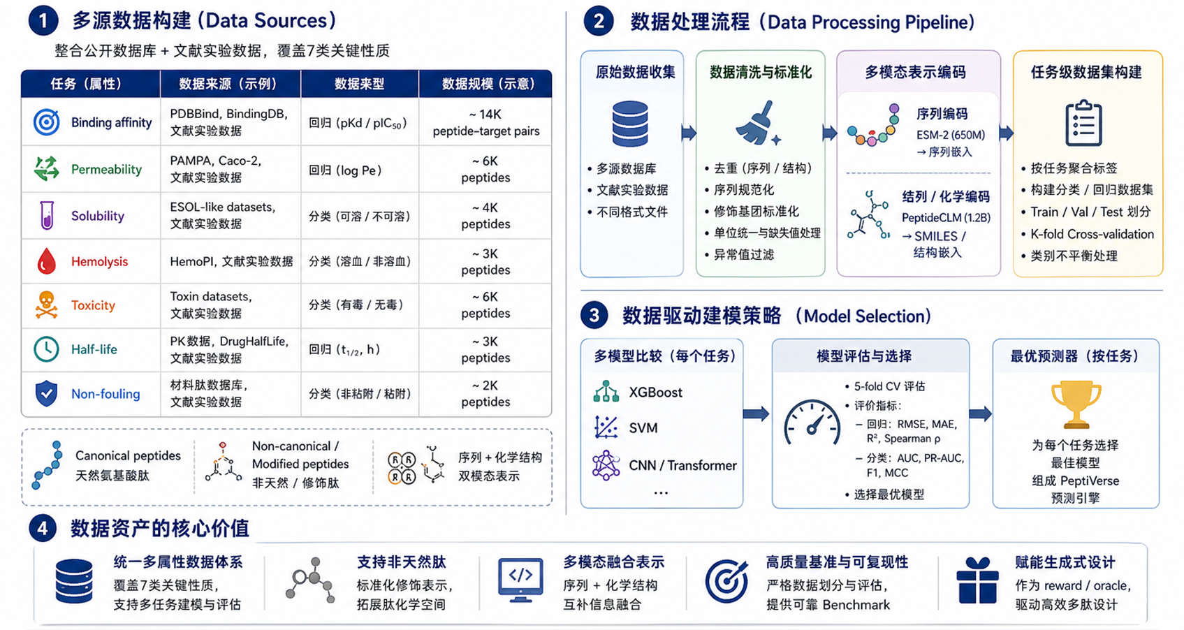
基于PeptiVerse深度学习模型的多肽ADMET性质预测工具,支持溶血性、溶解性、细胞穿透性、毒性、膜通透性、半衰期等多种性质的批量预测。输入支持标准氨基酸序列和 SMILES 化学结构两种格式,适用于线性肽、环肽及修饰肽的虚拟筛选与性质评估。
适用场景
输入的FASTA 格式多肽序列文件:
>id1
ZCVBDSWERTA
>id2
WERTAZCV
预测属性名称,必填,支持多选。
是否计算预测不确定性。启用后输出结果包含不确定性估计值,有助于评估预测可靠性。
预测结果的输出文件路径,默认输出为 results.csv。
输入的多肽文件,支持 SMILES 格式:
N[C@@H](CC(C)C)C(=O)N[C@@H](CC(=O)N)C(=O)N[C@@H](CCC(=O)N)C(=O)N[C@@H](CC(=CN2)C1=C2C=CC=C1)C(=O)N[C@@H](CC(=O)O)C(=O)N[C@@H](CO)C(=O)N[C@@H](CC(=CN2)C1=C2C=CC=C1)C(=O)N[C@@H](Cc1ccccc1)C(=O)N[C@@H](CC(=O)N)C(=O)N[C@@H](CCC(=O)O)C(=O)N[C@@H](CCSC)C(=O)N[C@@H]([C@H](CC)C)C(=O)N[C@@H](CCC(=O)N)C(=O)N[C@@H](CCCCN)C(=O)N[C@@H]([C@H](O)C)C(=O)NCC(=O)N[C@@H](CO)C(=O)O
预测属性名称,必填,支持多选。
是否计算预测不确定性。启用后输出结果包含不确定性估计值,有助于评估预测可靠性。
预测结果的输出文件路径,默认输出为 results.csv。
输出结果包括 results.csv 预测结果表格,包含每条多肽的各项预测性质及对应的不确定性。
results.csv 包含信息如下:
| 列名 | 说明 |
|---|---|
id |
多肽标识符,与输入文件中的 id 对应 |
halflife |
回归任务,血清半衰期预测值,反映多肽在体内的稳定性,越大越稳定。单位:小时 (h) |
halflife_uncertainty_type |
半衰期不确定性的计算类型标识 |
toxicity |
分类任务(概率值),毒性预测值,评估多肽的潜在毒性风险,越小越安全。范围 [0, 1],无量纲 |
toxicity_uncertainty_type |
毒性不确定性的计算类型标识 |
hemolysis |
分类任务(概率值),溶血性预测值,评估破坏红细胞风险(HC50 < 100 μM 为溶血),越小越安全。范围 [0, 1],无量纲 |
hemolysis_uncertainty_type |
溶血性不确定性的计算类型标识 |
permeability_pampa |
回归任务,PAMPA 平行人工膜通透性预测值,反映被动跨膜扩散能力,越大通透性越好。好:> -6.0单位:log Pe (log₁₀ cm/s),范围约 -9 ~ -5 |
permeability_pampa_uncertainty |
PAMPA 通透性预测的共形预测区间。格式 (lo, hi) 元组 |
permeability_pampa_uncertainty_type |
PAMPA 通透性不确定性的计算类型标识 |
nf |
分类任务(概率值),非特异性吸附(抗污性)预测值,评估非特异性相互作用倾向,越小抗污性越好。范围 [0, 1],无量纲 |
nf_uncertainty |
非特异性吸附预测的二元预测熵。范围 [0, ln2 ≈ 0.693] |
nf_uncertainty_type |
非特异性吸附不确定性的计算类型标识 |
solubility |
分类任务(概率值),溶解性预测值,反映多肽在水相环境中的溶解能力,越大水溶性越好。范围 [0, 1],无量纲 |
solubility_uncertainty_type |
溶解性不确定性的计算类型标识 |
permeability_penetrance |
分类任务(概率值),细胞穿透性预测值,评估多肽进入细胞膜的能力,越大穿透能力越强。范围 [0, 1],无量纲 |
permeability_penetrance_uncertainty |
细胞穿透性预测的二元预测熵。范围 [0, ln2 ≈ 0.693] |
permeability_penetrance_uncertainty_type |
细胞穿透性不确定性的计算类型标识 |
permeability_caco2 |
回归任务,Caco-2 细胞通透性预测值,反映肠道吸收潜力,越大吸收越好。单位:log Pe (log₁₀ cm/s),范围约 -9 ~ -5 |
permeability_caco2_uncertainty |
Caco-2 通透性预测的共形预测区间。格式 (lo, hi) 元组 |
permeability_caco2_uncertainty_type |
Caco-2 通透性不确定性的计算类型标识 |
| 类型标识 | 含义 | 取值范围 | 解读 |
|---|---|---|---|
binary_predictive_entropy |
二元预测熵(基于集成模型预测分布) | [0, ln2 ≈ 0.693] | 越接近 0 越确定,越接近 0.693 越接近不确定 |
ensemble_predictive_entropy |
集成预测熵(多分类) | [0, ln(n)] | 同上,n 为类别数 |
binary_predictive_entropy_single_model |
单模型二元预测熵 | [0, ln2 ≈ 0.693] | 仅基于单一模型,可信度低于集成版本 |
conformal_prediction_interval |
共形预测区间 (lo, hi) | 无界 | 真实值有较高概率(如 90%)落在区间内,区间越窄越可信 |
unavailable (no seed ensemble found) |
无集成模型可用 | — | 无法量化不确定性,对该字段需谨慎 |
unavailable (no MAPIE bundle for XGBoost regression) |
XGBoost 回归无 MAPIE 配套 | — | 无共形区间可用,对该字段需谨慎 |
注意:不确定性指标仅在 Uncertainty 选择 true 时输出。
A deep learning-based multi-property prediction tool for peptides, supporting batch prediction of properties including hemolysis, solubility, cell penetration, toxicity, membrane permeability, half-life, and binding affinity. Input supports both standard amino acid sequences and SMILES chemical structure formats, making it suitable for virtual screening and property evaluation of linear peptides, cyclic peptides, and modified peptides.
Use Cases
Input peptide sequence file in FASTA format:
>id1
ZCVBDSWERTA
>id2
WERTAZCV
The properties to predict. Required; multiple selections supported.
Input peptide file in SMILES format:
N[C@@H](CC(C)C)C(=O)N[C@@H](CC(=O)N)C(=O)...
The properties to predict. Required; multiple selections supported.
Target Sequence is provided, this property will be automatically skipped.Whether to calculate prediction uncertainty. When enabled, the output includes uncertainty estimates to help assess prediction reliability.
Output file path for prediction results. Defaults to results.csv.
The output is a results.csv prediction table containing the predicted properties and corresponding uncertainty estimates for each peptide.
| Column Name | Description |
|---|---|
id |
Peptide identifier, corresponding to the id in the input file |
halflife |
Regression task: predicted serum half-life value, reflecting peptide stability in vivo; higher values indicate greater stability. Unit: hours (h) |
halflife_uncertainty_type |
Uncertainty type identifier for half-life prediction |
toxicity |
Classification task (probability value): predicted toxicity score, assessing potential toxic risk of the peptide; lower values are safer. Range: [0, 1], dimensionless |
toxicity_uncertainty_type |
Uncertainty type identifier for toxicity prediction |
hemolysis |
Classification task (probability value): predicted hemolytic activity, assessing risk of red blood cell destruction (HC50 < 100 μM indicates hemolysis); lower values are safer. Range: [0, 1], dimensionless |
hemolysis_uncertainty_type |
Uncertainty type identifier for hemolysis prediction |
permeability_pampa |
Regression task: predicted PAMPA (Parallel Artificial Membrane Permeability Assay) value, reflecting passive trans-membrane diffusion ability; higher values indicate better permeability. Good: > -6.0. Unit: log Pe (log₁₀ cm/s), range approximately -9 ~ -5 |
permeability_pampa_uncertainty |
Conformal prediction interval for PAMPA permeability. Format: (lo, hi) tuple |
permeability_pampa_uncertainty_type |
Uncertainty type identifier for PAMPA permeability prediction |
nf |
Classification task (probability value): predicted non-specific adsorption (antifouling property) score, assessing tendency for non-specific interactions; lower values indicate better antifouling. Range: [0, 1], dimensionless |
nf_uncertainty |
Binary predictive entropy for non-specific adsorption prediction. Range: [0, ln2 ≈ 0.693] |
nf_uncertainty_type |
Uncertainty type identifier for non-specific adsorption prediction |
solubility |
Classification task (probability value): predicted solubility score, reflecting peptide dissolution ability in aqueous environment; higher values indicate better water solubility. Range: [0, 1], dimensionless |
solubility_uncertainty_type |
Uncertainty type identifier for solubility prediction |
permeability_penetrance |
Classification task (probability value): predicted cell penetration ability, assessing peptide capacity to enter cell membrane; higher values indicate stronger penetration. Range: [0, 1], dimensionless |
permeability_penetrance_uncertainty |
Binary predictive entropy for cell penetration prediction. Range: [0, ln2 ≈ 0.693] |
permeability_penetrance_uncertainty_type |
Uncertainty type identifier for cell penetration prediction |
permeability_caco2 |
Regression task: predicted Caco-2 cell permeability value, reflecting intestinal absorption potential; higher values indicate better absorption. Unit: log Pe (log₁₀ cm/s), range approximately -9 ~ -5 |
permeability_caco2_uncertainty |
Conformal prediction interval for Caco-2 permeability. Format: (lo, hi) tuple |
permeability_caco2_uncertainty_type |
Uncertainty type identifier for Caco-2 permeability prediction |
| Type Identifier | Meaning | Value Range | Interpretation |
|---|---|---|---|
binary_predictive_entropy |
Binary predictive entropy (based on ensemble model prediction distribution) | [0, ln2 ≈ 0.693] | Closer to 0 indicates higher certainty; closer to 0.693 indicates greater uncertainty |
ensemble_predictive_entropy |
Ensemble predictive entropy (multiclass) | [0, ln(n)] | Same as above; n is the number of classes |
binary_predictive_entropy_single_model |
Single-model binary predictive entropy | [0, ln2 ≈ 0.693] | Based on a single model only; lower credibility than ensemble version |
conformal_prediction_interval |
Conformal prediction interval (lo, hi) | Unbounded | True value has high probability (e.g., 90%) of falling within the interval; narrower intervals are more credible |
unavailable (no seed ensemble found) |
No ensemble model available | — | Unable to quantify uncertainty; use caution when interpreting this field |
unavailable (no MAPIE bundle for XGBoost regression) |
XGBoost regression has no MAPIE support | — | No conformal interval available; use caution when interpreting this field |
Note: Uncertainty columns are only included in the output when Uncertainty is set to true.

从输入 PDB 文件中自动提取抗体 Fv 区域及邻近分子片段,生成包含 Fv 与伙伴链的截断 PDB 和 Fv 序列文件,并进行界面(interface)和氢键(hydrogen bond)相互作用计算。
核心技术
适用场景
输入的抗体 PDB 结构文件,需包含完整的抗体结构及可能结合的抗原、配体或其他分子。输入时请限制抗体及其相互作用的对象是一对一的,例如一个轻重连构成的抗体对应抗原,而非多个抗体对应一个抗原
Fv 编号方案,用于确定 CDR 位置和 Fv 截断点。
Fv 与邻近分子的接触截止距离,用于识别需要保留的伙伴链。单位 Å,默认 10.0 Å。
输出结果包括:
| 文件名 | 说明 |
|---|---|
extracted_fv.pdb |
截断后的 Fv 及邻近伙伴链的 PDB 结构文件 |
extracted_fv.fasta |
提取的 Fv 氨基酸序列,可用于后续人源化流程 |
interface_cb.json |
界面相互作用计算结果,包含原子/残基级别的接触信息 |
hydrogen_bond.json |
氢键计算结果,包含供体-受体对、距离和角度信息 |
extracted_HL.pdb |
截断后Fv的PDB 结构文件 |
Automatically extracts the antibody Fv region and neighboring molecular fragments from an input PDB file, generates a truncated PDB containing Fv with partner chains and an Fv sequence file, and calculates interface and hydrogen bond interactions.
Core Technologies
Use Cases
Input antibody PDB structure file, which should contain the complete antibody structure and any bound antigens, ligands, or other molecules.
Fv numbering scheme used to determine CDR positions and Fv truncation points.
Contact cutoff distance between Fv and neighboring molecules for identifying partner chains to retain. Unit: Å, default 10.0 Å.
The output includes the following files:
| File Name | Description |
|---|---|
extracted_fv.pdb |
Truncated PDB structure file containing Fv and neighboring partner chains |
extracted_fv.fasta |
Extracted Fv amino acid sequence, available for downstream humanization workflows |
interface_cb.json |
Interface interaction calculation results, including atom/residue-level contact information |
hydrogen_bond.json |
Hydrogen bond calculation results, including donor-acceptor pairs, distances, and angles |
extracted_HL.pdb |
PDB structure file of the truncated Fv |

对 Immunogenicity Prediction (AlphaMHC v3.0 beta)和 Immunogenicity Prediction (WeADApt v4.1.0)、Immunogenicity Prediction (WeADApt v4.2)、Immunogenicity Prediction (WeADApt v4.3) 四个免疫原性评估模块的结果进行汇总,生成分子和表位级别的整合报告。该模块为流程编排组件,需配合上游免疫原性预测模块使用。
基础输入目录,仅作为省略的输入文件参数的默认路径前缀。
FASTA 格式的氨基酸序列文件。
AlphaMHC v3.0 分子评分 CSV 文件。
AlphaMHC v3.0 表位评分 CSV 文件。
WeAdapt v4.1 分子评分 CSV 文件。
WeAdapt v4.1 表位评分 CSV 文件。
WeAdapt v4.2 分子评分 CSV 文件。
WeAdapt v4.2 表位评分 CSV 文件。
WeAdapt v4.3 分子评分 CSV 文件。
WeAdapt v4.3 表位评分 CSV 文件。
分子汇总 CSV 输出路径。
表位汇总 CSV 输出路径。
记录级错误 CSV 输出路径。
输出结果包括:
| 文件名 | 说明 |
|---|---|
molecule_summary.csv |
分子级别汇总结果,整合各模块的分子评分 |
epitope_summary.csv |
表位级别汇总结果,整合各模块的表位评分 |
errors.csv |
记录级错误日志,汇总处理过程中的异常信息 |
molecule_summary.csv文件包含信息如下:
| 列名 | 说明 |
|---|---|
molecule |
蛋白质分子名称(取自 FASTA 和 CSV 中的 Protein ID) |
AlphaMHC_v3.0_score |
AlphaMHC v3.0 模块给出的分子级别评分 |
WeAdapt_v4.1_score |
WeAdapt v4.1 模块给出的分子级别评分 |
WeAdapt_v4.2_score |
WeAdapt v4.2 模块给出的分子级别评分 |
WeAdapt_v4.3_score |
WeAdapt v4.3 模块给出的分子级别评分 |
mean_score(v4) |
WeAdapt 三个版本(v4.1 / v4.2 / v4.3)评分的均值,AlphaMHC 不参与统计 |
max_score(v4) |
WeAdapt 三个版本评分的最大值 |
min_score(v4) |
WeAdapt 三个版本评分的最小值 |
epitope_summary.csv文件包含信息如下:
| 列名 | 说明 |
|---|---|
molecule |
蛋白质分子名称 |
chain |
序列 ID(chain 名称) |
epitope_id |
表位编号,格式 Epitope_001,按分子内出现顺序递增 |
epitope_position |
表位在序列上的区间,格式 begin-end(1-based) |
epitope |
代表性表位肽段序列(优先取 FASTA 对应区间子串,否则取聚类中最长肽段) |
mean_score(v4) |
聚类中 WeAdapt 三版评分的均值(AlphaMHC 不参与统计) |
max_score(v4) |
聚类中 WeAdapt 三版评分的最大值 |
min_score(v4) |
聚类中 WeAdapt 三版评分的最小值 |
AlphaMHC_v3.0_score |
聚类中 AlphaMHC v3.0 表位的最高评分 |
WeAdapt_v4.1_score |
聚类中 WeAdapt v4.1 表位的最高评分 |
WeAdapt_v4.2_score |
聚类中 WeAdapt v4.2 表位的最高评分 |
WeAdapt_v4.3_score |
聚类中 WeAdapt v4.3 表位的最高评分 |
AlphaMHC_v3.0_HLA |
AlphaMHC v3.0 模块关联的 HLA 等位基因(该模块无 HLA 数据,始终为 /) |
WeAdapt_v4.1_HLA |
WeAdapt v4.1 模块关联的 HLA 等位基因,分号分隔 |
WeAdapt_v4.2_HLA |
WeAdapt v4.2 模块关联的 HLA 等位基因,分号分隔 |
WeAdapt_v4.3_HLA |
WeAdapt v4.3 模块关联的 HLA 等位基因,分号分隔 |
overlapping_HLA |
各模块 HLA 集合的交集(至少 2 个模块有 HLA 数据时才计算),无交集或数据不足时为 / |
Aggregates results from four immunogenicity assessment modules ( Immunogenicity Prediction (AlphaMHC v3.0 beta) and Immunogenicity Prediction (WeADApt v4.1.0)、Immunogenicity Prediction (WeADApt v4.2)、Immunogenicity Prediction (WeADApt v4.3)) to generate integrated molecule-level and epitope-level reports. This module is a workflow orchestration component and must be used in conjunction with upstream immunogenicity prediction modules.
Base input directory used only as the default path prefix for omitted input file arguments.
Amino acid sequence file in FASTA format.
AlphaMHC v3.0 molecule score CSV file.
AlphaMHC v3.0 epitope score CSV file.
WeAdapt v4.1 molecule score CSV file.
WeAdapt v4.1 epitope score CSV file.
WeAdapt v4.2 molecule score CSV file.
WeAdapt v4.2 epitope score CSV file.
WeAdapt v4.3 molecule score CSV file.
WeAdapt v4.3 epitope score CSV file.
Molecule summary CSV output path.
Epitope summary CSV output path.
Record-level error CSV output path.
The output includes the following files:
| File Name | Description |
|---|---|
molecule_summary.csv |
Molecule-level summary integrating scores from all modules |
epitope_summary.csv |
Epitope-level summary integrating scores from all modules |
errors.csv |
Record-level error log summarizing exceptions during processing |
The molecule_summary.csv file contains the following columns:
| Column | Description |
|---|---|
molecule |
Protein molecule name (taken from the Protein ID in FASTA and CSV) |
AlphaMHC_v3.0_score |
Molecule-level score from the AlphaMHC v3.0 module |
WeAdapt_v4.1_score |
Molecule-level score from the WeAdapt v4.1 module |
WeAdapt_v4.2_score |
Molecule-level score from the WeAdapt v4.2 module |
WeAdapt_v4.3_score |
Molecule-level score from the WeAdapt v4.3 module |
mean_score(v4) |
Mean of the three WeAdapt version scores (v4.1 / v4.2 / v4.3); AlphaMHC is excluded |
max_score(v4) |
Maximum of the three WeAdapt version scores |
min_score(v4) |
Minimum of the three WeAdapt version scores |
The epitope_summary.csv file contains the following columns:
| Column | Description |
|---|---|
molecule |
Protein molecule name |
chain |
Sequence ID (chain name) |
epitope_id |
Epitope identifier, formatted as Epitope_001, incrementing in order of appearance within the molecule |
epitope_position |
Epitope interval on the sequence, formatted as begin-end (1-based) |
epitope |
Representative epitope peptide sequence (preferentially taken from the corresponding FASTA subsequence; otherwise the longest peptide in the cluster) |
mean_score(v4) |
Mean of the three WeAdapt version scores within the cluster (AlphaMHC is excluded) |
max_score(v4) |
Maximum of the three WeAdapt version scores within the cluster |
min_score(v4) |
Minimum of the three WeAdapt version scores within the cluster |
AlphaMHC_v3.0_score |
Highest AlphaMHC v3.0 epitope score within the cluster |
WeAdapt_v4.1_score |
Highest WeAdapt v4.1 epitope score within the cluster |
WeAdapt_v4.2_score |
Highest WeAdapt v4.2 epitope score within the cluster |
WeAdapt_v4.3_score |
Highest WeAdapt v4.3 epitope score within the cluster |
AlphaMHC_v3.0_HLA |
HLA allele associated with the AlphaMHC v3.0 module (this module has no HLA data, always /) |
WeAdapt_v4.1_HLA |
HLA allele(s) associated with the WeAdapt v4.1 module, semicolon-separated |
WeAdapt_v4.2_HLA |
HLA allele(s) associated with the WeAdapt v4.2 module, semicolon-separated |
WeAdapt_v4.3_HLA |
HLA allele(s) associated with the WeAdapt v4.3 module, semicolon-separated |
overlapping_HLA |
Intersection of HLA sets across modules (computed only when at least 2 modules have HLA data); / when there is no overlap or insufficient data |
基于 ANARCI 和 mafft 的抗体序列编号工具,支持 FV 和 FC 批量编号。
Antibody Numbering 是一个抗体序列编号工具,用于将抗体氨基酸序列映射到标准化编号体系。编号后的序列具有统一的位置参照,使得不同抗体之间的同源比对、CDR 精确定位、突变分析等工作成为可能。
抗体序列的氨基酸残基数因克隆不同而差异较大,直接比较两条原始序列很难确定哪些位置是同源的。编号方案通过为每个残基赋予标准化编号来解决这个问题,使研究人员能够准确识别 CDR 和 FR 的边界。
适用场景:
FV 编号使用 ANARCI 引擎,自动识别输入序列中的可变区结构域,支持单条序列中包含多个结构域的情况。编号结果包含每个残基的标准化编号、CDR/FR 区域标注及链类型判定。支持 IMGT、Kabat、Chothia、Martin、AHo、CCG 等方案。
FC 编号使用 mafft 多序列比对引擎,将输入序列与已知恒定区模板进行比对,通过匹配率判定同种型和亚型。适用于同型鉴定、Fc 工程改造等下游分析。支持 EU 和 Kabat 方案。
每个编号方案生成独立的 JSON 和 CSV 结果文件。FV 还会生成未覆盖片段 FASTA,FC 还会生成模板匹配率 CSV。summary.jsonl 包含各方案的处理统计,failed.fasta 收集编号失败的序列。
该模式针对抗体的Fv区序列(包括重链 VH 和轻链 VL),通过指定编号规则(如 Kabat、Chothia、或 IMGT等)对氨基酸残基进行标准化编号。
上传需要进行抗体编号的氨基酸序列文件。支持批量提交多条序列,文件内容应使用 FASTA 格式。
可变区编号规则,支持IMGT、Kabat、Chothia、Martin、AHo、CCG可多选。
通常用于抗体的EU、Kabat标准化编号。
上传需要进行抗体恒定区编号的氨基酸序列文件。支持批量提交多条序列,文件内容应使用 FASTA 格式。
恒定区编号规则:eu,kabat。默认为eu。
输出结果包含以下文件:
| 文件名 | 说明 |
|---|---|
summary.jsonl |
汇总每个编号方案的处理统计,包括成功、未匹配、失败的序列数量 |
failed.fasta |
保存编号失败的原始序列 |
output_{scheme}.json |
抗体编号结果文件,json格式,按不同编号方案分别生成(如 Chothia、IMGT、Kabat、Martin),包含 residue 编号、区域标注和链类型等信息 |
output_{scheme}.csv |
抗体编号结果文件,csv格式,按不同编号方案分别生成(如 Chothia、IMGT、Kabat、Martin),包含 residue 编号、区域标注和链类型等信息 |
non_fv_{scheme}.fasta |
未被识别为 FV 可变区的剩余片段(仅 FV 编号) |
output_{scheme}_match_rate.csv |
输入序列与各 FC 模板的匹配率(仅 FC 编号) |
FV Numbering模式输出的output_{scheme}.csv文件包含信息如下:
| 列名 | 说明 |
|---|---|
| molecule | 抗体链类型(VH = 重链可变区,VL = 轻链可变区) |
| residue | 氨基酸残基(单字母表示,如 E = 谷氨酸) |
| chain_type | 链的具体类型(如 VK = κ轻链,VL = λ轻链,VH = 重链) |
| species | 抗体来源物种(如 human、mouse) |
| is_cdr | 是否属于 CDR 区(True = CDR,False = 框架区 FR) |
| loc | 在原始序列中的位置(从1开始计数) |
| numbering | 抗体编号体系中的位置(如 IMGT/Kabat 编号) |
| insertion | 插入位点标记(如 A、B;无则为空) |
| region | 所属区域(FR1、CDR1、FR2、CDR2、FR3、CDR3、FR4) |
| domain | 所属结构域编号(用于区分多结构域抗体) |
FC Numbering模式输出的output_{scheme}.csv文件包含信息如下:
| 列名 | 含义 |
|---|---|
| molecule | 抗体分子ID |
| chain_type | 抗体链类型或来源注释,例如 Mouse IgG2a(小鼠IgG2a亚型) |
| position | EU编号体系中的残基编号(EU index位置) |
| region | 抗体结构区域标注(如 FR、CDR、hinge 等;“-”表示未归类或非关键区) |
| ref_residue | 参考序列(template / germline / wild-type)上的氨基酸 |
| residue | 实际观测或目标结构中的氨基酸 |
| mutation | 突变信息(ref → observed)。“-”表示无突变(完全一致) |
FC Numbering模式输出的output_{scheme}_match_rate.csv文件包含信息如下:
| 列名 | 含义 |
|---|---|
| Chain | 抗体链标识 |
| Template | 用于比对的模板类型(如 IgG1_H 表示 IgG1 重链模板) |
| MatchRate_CH1 | CH1结构域的匹配率(序列或结构相似度) |
| MatchRate_Hinge | Hinge(铰链区)的匹配率 |
| MatchRate_CH2 | CH2结构域的匹配率 |
| MatchRate_CH3 | CH3结构域的匹配率 |
| MatchRate_Global | 全局匹配率(整体结构/序列相似度) |
An antibody sequence numbering tool based on ANARCI and mafft, supporting batch numbering for FV and FC regions.
Antibody Numbering is a tool that maps antibody amino acid sequences to standardized numbering schemes. Numbered sequences share a unified positional reference, enabling homologous alignment across different antibodies, precise CDR localization, and mutation analysis.
The number of amino acid residues in antibody sequences varies widely across clones, making it difficult to identify homologous positions by comparing raw sequences directly. Numbering schemes resolve this by assigning each residue a standardized identifier, allowing researchers to accurately delineate CDR and FR boundaries.
Use cases:
The FV numbering module uses the ANARCI engine to automatically identify variable-region domains in input sequences, supporting cases where a single sequence contains multiple domains. Results include standardized residue numbering, CDR/FR region annotations, and chain-type classification. Supported schemes include IMGT, Kabat, Chothia, North, Martin, AHo, and CCG.
The FC numbering module uses the mafft multiple-sequence-alignment engine to align input sequences against known constant-region templates, determining isotype and subtype by match rate. Applicable for isotype identification and Fc engineering downstream analyses. Supported schemes include EU and Kabat.
Each numbering scheme generates independent JSON and CSV result files. FV numbering also produces an unassigned-segment FASTA file, and FC numbering produces a template match-rate CSV. summary.jsonl contains per-scheme processing statistics, and failed.fasta collects sequences that failed numbering.
This mode targets Fv-region sequences of antibodies (including heavy chain VH and light chain VL), applying a standardized numbering scheme (e.g., Kabat, Chothia, IMGT) to amino acid residues.
Upload the amino acid sequence file for antibody numbering. Batch submission of multiple sequences is supported; file content must be in FASTA format.
Variable-region numbering rules. Supports IMGT, Kabat, Chothia, Martin, AHo, and CCG. Multiple selection is allowed.
Commonly used for standardized EU and Kabat numbering of antibody constant regions.
Upload the amino acid sequence file for antibody constant-region numbering. Batch submission of multiple sequences is supported; file content must be in FASTA format.
Constant-region numbering rules: eu, kabat. Default is eu.
Output results include the following files:
| Filename | Description |
|---|---|
summary.jsonl |
Aggregated processing statistics for each numbering scheme, including counts of successful, unmatched, and failed sequences |
failed.fasta |
Raw sequences that failed numbering |
output_{scheme}.json |
Antibody numbering results in json format, generated per scheme (e.g., Chothia, IMGT, Kabat, Martin), containing residue numbering, region annotations, and chain-type information |
output_{scheme}.csv |
Antibody numbering results in csv format, generated per scheme (e.g., Chothia, IMGT, Kabat, Martin), containing residue numbering, region annotations, and chain-type information |
non_fv_{scheme}.fasta |
Remaining segments not identified as FV variable regions (FV numbering only) |
output_{scheme}_match_rate.csv |
Match rates between input sequences and each FC template (FC numbering only) |
The output_{scheme}.csv files produced by both FV Numbering modes contain the following columns:
| Column | Description |
|---|---|
| molecule | Antibody chain type (VH = heavy chain variable region, VL = light chain variable region) |
| residue | Amino acid residue (single-letter code, e.g., E = Glutamic acid) |
| chain_type | Specific chain type (e.g., VK = κ light chain, VL = λ light chain, VH = heavy chain) |
| species | Source species of the antibody (e.g., human, mouse) |
| is_cdr | Whether the residue belongs to a CDR region (True = CDR, False = framework region FR) |
| loc | Position in the original sequence (1-based index) |
| numbering | Position in the numbering scheme (e.g., IMGT/Kabat numbering) |
| insertion | Insertion marker (e.g., A, B; empty if none) |
| region | Belonging region (FR1, CDR1, FR2, CDR2, FR3, CDR3, FR4) |
| domain | Domain index (used to distinguish multi-domain antibodies) |
The output_{scheme}_match_rate.csv files produced by the FC Numbering mode contain the following columns:
| Column | Description |
|---|---|
| Chain | Antibody chain identifier |
| Template | Template type used for alignment (e.g., IgG1_H indicates an IgG1 heavy chain template) |
| MatchRate_CH1 | Match rate for the CH1 domain (sequence or structural similarity) |
| MatchRate_Hinge | Match rate for the Hinge region |
| MatchRate_CH2 | Match rate for the CH2 domain |
| MatchRate_CH3 | Match rate for the CH3 domain |
| MatchRate_Global | Global match rate (overall sequence/structural similarity) |
FC Numbering mode output output_{scheme}.csv contains the following fields:
| Column | Description |
|---|---|
| molecule | Antibody molecule ID |
| chain_type | Antibody chain type or source annotation, e.g., Mouse IgG2a subtype |
| position | Residue position in the EU numbering system (EU index position) |
| region | Structural region annotation (e.g., FR, CDR, hinge; “-” indicates unassigned or non-critical region) |
| ref_residue | Amino acid in the reference sequence (template / germline / wild-type) |
| residue | Amino acid observed in the target or input structure |
| mutation | Mutation annotation (ref → observed). “-” indicates no mutation (identical residue) |

基于 ANARCI 的抗体序列快速分类工具,将输入 FASTA 文件中的序列自动划分为可编号、不可编号和异常序列三类,并分别输出到独立的 FASTA 文件中。
核心技术
适用场景
输入的抗体氨基酸序列文件,需为标准 FASTA 格式,支持单条或多条序列。
注意:仅包含完整或可识别 Fv(可变区)结构域的序列才能被 ANARCI 正确编号。
ANARCI 编号方案,用于判定序列是否可被识别为抗体可变区并进行编号。
默认使用 IMGT。
可编号序列(即成功识别为 Fv 区域的序列)的输出文件路径。
这些序列包含可解析的抗体可变区结构域,可被 ANARCI 成功编号,并适用于下游分析(如 CDR 定位、人源化等)。
默认输出文件为 numberable.fasta。
不可编号序列的输出文件路径。
这些序列不包含可识别的 Fv 区域,或与标准抗体可变区差异过大,因此无法被 ANARCI 识别和编号。
默认输出文件为 unnumberable.fasta。
异常序列的输出文件路径。
这些序列存在格式错误(如 FASTA 不规范)、包含非标准氨基酸,或其他导致无法解析的问题。
默认输出文件为 invalid.fasta。
输出结果包括以下文件:
| 文件名 | 说明 |
|---|---|
numberable.fasta |
包含可被 ANARCI 识别为 Fv 区域并成功编号的序列,可直接用于下游编号与抗体工程分析 |
unnumberable.fasta |
不包含可识别 Fv 区域或偏离标准抗体结构的序列,无法进行编号 |
invalid.fasta |
输入异常序列,包括格式错误或非法字符等,未参与编号流程 |
A rapid antibody sequence classification tool based on ANARCI that automatically partitions sequences from an input FASTA file into three categories: numberable, unnumberable, and invalid, exporting each to separate FASTA files.
Core Technologies
Use Cases
Input antibody amino acid sequence file in standard FASTA format, supporting single or multiple sequences.
Note: Only sequences containing complete or recognizable Fv (variable region) domains can be correctly numbered by ANARCI.
ANARCI numbering scheme used to determine whether a sequence can be recognized as an antibody variable region and subsequently numbered.
Default: IMGT.
Output file path for numberable sequences (i.e., sequences successfully identified as Fv regions).
These sequences contain parseable antibody variable region domains that can be successfully numbered by ANARCI, and are suitable for downstream analyses (e.g., CDR localization, humanization, etc.).
Default output file: numberable.fasta.
Output file path for unnumberable sequences.
These sequences do not contain recognizable Fv regions or deviate too far from standard antibody variable regions, and therefore cannot be recognized or numbered by ANARCI.
Default output file: unnumberable.fasta.
Output file path for invalid sequences.
These sequences have formatting errors (e.g., non-standard FASTA), contain non-standard amino acids, or have other issues that prevent parsing.
Default output file: invalid.fasta.
The output includes the following files:
| Filename | Description |
|---|---|
numberable.fasta |
Sequences recognized by ANARCI as Fv regions and successfully numbered; ready for downstream numbering and antibody engineering analysis |
unnumberable.fasta |
Sequences without recognizable Fv regions or that deviate from standard antibody structures; cannot be numbered |
invalid.fasta |
Abnormal input sequences, including format errors or illegal characters; excluded from the numbering workflow |
Split Antibody Chain 是一个用于拆分抗体链的工具,能够将混合的抗体序列分离为重链、轻链和非抗体序列。
核心思想
本项目采用 基于抗体编号方案的链分类 策略:
该流程以"基于 IMGT/Kabat/Chothia 编号方案的抗体链分类"为核心,实现抗体序列的自动化拆分和分类功能。
输入文件路径,FASTA 格式,为必选参数。
注意:仅包含完整或可识别 Fv(可变区)结构域的序列才能被 ANARCI 识别为抗体重链和轻链。
抗体编号方案,可选值包括 imgt、kabat 或 chothia。该方案用于链分类的标准依据。
输出包含抗体重链序列的文件名称
输出包含抗体轻链序列的文件名称
输出包含非抗体序列的文件名称
输出结果包括以下 FASTA 格式文件:
| 输出文件名称 | 说明 |
|---|---|
| heavy_chain.fasta | 按照指定编号方案识别的重链序列 |
| light_chain.fasta | 按照指定编号方案识别的轻链序列 |
| non_antibody.fasta | 未识别为抗体的序列 |
所有输出文件均为 FASTA 格式,每条记录包含序列标识符和氨基酸序列。
Split Antibody Chain is a tool for splitting mixed antibody sequences into heavy chains, light chains, and non-antibody sequences.
Core concept
This tool adopts a numbering-scheme-based chain classification strategy:
The workflow centers on “antibody chain classification based on IMGT/Kabat/Chothia numbering schemes,” achieving automated splitting and classification of antibody sequences.
Input file path in FASTA format. Required.
Note: Only sequences containing complete or recognizable Fv (variable region) domains can be recognized by ANARCI as antibody heavy or light chains.
Antibody numbering scheme. Supported values: imgt, kabat, or chothia. This scheme serves as the standard basis for chain classification.
Output filename for sequences identified as antibody heavy chains.
Output filename for sequences identified as antibody light chains.
Output filename for sequences identified as non-antibody sequences.
Output files include the following FASTA-format files:
| Output Filename | Description |
|---|---|
heavy_chain.fasta |
Heavy chain sequences identified according to the specified numbering scheme. |
light_chain.fasta |
Light chain sequences identified according to the specified numbering scheme. |
non_antibody.fasta |
Sequences not recognized as antibodies. |
All output files are in FASTA format; each record contains a sequence identifier and the amino acid sequence.

基于 MolPK 模型的药代动力学(PK)参数批量预测工具。利用预训练深度学习模型,从小分子结构(SMILES)及实验条件(物种、给药途径、剂量)预测 PK 参数,支持多种输入格式和灵活的批处理场景。
核心技术
适用场景
输入的待预测文件,支持 .smi(SMILES 文本)、.csv(表格)或 .sdf(结构文件)格式。为必填参数。
实验物种,可选值为 rat(大鼠)、mou(小鼠)、dog(犬)、hum(人)。用于指定 PK 预测对应的物种背景。
给药途径,可选值为 iv(静脉注射)、po(口服)。不同给药途径对 PK 曲线有显著影响。
给药剂量,单位为 mg/kg。用于指定预测时对应的剂量条件。
预测结果的 CSV 输出路径。默认输出为 pred_pk_value.csv。
带 PK 预测属性的 SDF 结构文件输出路径。默认输出为 pred_with_pk_value.sdf。
当输入为 CSV 文件时,指定包含 SMILES 字符串的列名。
当输入为 CSV 文件时,指定包含物种信息的列名。
当输入为 CSV 文件时,指定包含给药途径信息的列名。
当输入为 CSV 文件时,指定包含剂量信息的列名。
输出结果包括:
| 文件名 | 说明 |
|---|---|
pred_pk_value.csv |
预测的 PK 参数表格,包含每个分子的预测值及输入条件 |
pred_with_pk_value.sdf |
带 PK 预测属性的分子结构文件,可直接用于结构查看和进一步分析 |
输出的预测结果文件文件pred_pk_value.csv:
| 列名 | 说明 |
|---|---|
| _smi_line | 原始输入的 SMILES 行字符串(通常包含分子结构及附加标识信息) |
| SMILES | 分子的标准 SMILES 表示,用于描述化学结构 |
| Species | 实验物种(如 human、mouse、rat 等) |
| Route | 给药途径(如 IV、PO 等) |
| Dose (mg/kg) | 给药剂量,单位为 mg/kg |
| CL (mL/min/kg) | 清除率(Clearance),单位为 mL/min/kg,表示单位时间内药物从体内被清除的能力 |
| Vd (L/kg) | 表观分布容积(Volume of distribution),单位为 L/kg,反映药物在体内的分布范围 |
| AUC (ng·h/mL) | 曲线下面积(Area Under the Curve),单位为 ng·h/mL,表示药物暴露量 |
| T1/2 (h) | 半衰期(Half-life),单位为小时,表示药物浓度降低一半所需时间 |
A batch pharmacokinetic (PK) parameter prediction tool . Utilizes a pretrained deep learning model to predict PK parameters from molecular structures (SMILES) and experimental conditions (species, administration route, dose), supporting multiple input formats and flexible batch processing scenarios.
Core Technologies
Use Cases
Input file for prediction, supporting .smi (SMILES text), .csv (table), or .sdf (structure file) formats. This is a required parameter.
Experimental species, with options rat, mou (mouse), dog, or hum (human). Specifies the species background for PK prediction.
Administration route, with options iv (intravenous) or po (oral). Different routes significantly affect PK profiles.
Administration dose in mg/kg. Specifies the dose condition for prediction.
Output CSV path for prediction results. Default: pred_pk_value.csv.
Output SDF structure file path with PK prediction attributes. Default: pred_with_pk_value.sdf.
When input is a CSV file, specifies the column name containing SMILES strings.
When input is a CSV file, specifies the column name containing species information.
When input is a CSV file, specifies the column name containing administration route information.
When input is a CSV file, specifies the column name containing dose information.
The output includes the following files:
| File Name | Description |
|---|---|
pred_pk_value.csv |
Predicted PK parameter table containing predicted values and input conditions for each molecule |
pred_with_pk_value.sdf |
Molecular structure file with PK prediction attributes, suitable for structure viewing and further analysis |
The predicted results are output to pred_pk_value.csv:
| Column Name | Description |
|---|---|
| _smi_line | Original input SMILES line (may include structure and additional identifiers) |
| SMILES | Standard SMILES representation of the molecule |
| Species | Experimental species (e.g., human, mouse, rat) |
| Route | Administration route (e.g., IV, PO) |
| Dose (mg/kg) | Administered dose in mg/kg |
| CL (mL/min/kg) | Clearance, expressed in mL/min/kg, indicating the rate of drug elimination |
| Vd (L/kg) | Volume of distribution, in L/kg, reflecting the extent of drug distribution in the body |
| AUC (ng·h/mL) | Area Under the Curve, representing overall drug exposure |
| T1/2 (h) | Half-life, in hours, indicating the time required for the drug concentration to decrease by half |

蛋白进化分析,快速找到能够协同作用的多重突变组合。基于MULTI-evolve框架实现,面向蛋白工程中的候选突变发现与组合优化,提供单点突变与多点突变两种工作模式:前者利用蛋白语言模型进行零样本评估,快速发现潜在有利的单点突变;后者基于实验测得的突变数据训练监督模型,并在候选突变池上进一步搜索高阶组合突变。该流程将蛋白语言模型、表观互作(epistasis)建模和后续实验构建衔接为一套端到端方案;其中单点突变部分实际整合了 5 个 ESM-1v 模型(esm1v_t33_650M_UR90S_1-5)、1 个 ESM-2 3B 模型(esm2_t36_3B_UR50D),以及结构感知的 ESM-IF1,多点突变部分则以全连接神经网络为核心预测器来学习序列与性质之间的映射。

使用流程:
1,计算步骤,先使用单点突变模式,获取优势单点突变(一般选择排名靠前的15-20个)
2,湿实验步骤,对第一步选择的单点突变,及其所有两点突变的组合(100~200个组合),进行湿实验验证,获取突变对应的湿实验数据,请使用性质数据的比值(Fold-Change,FC值),即: 突变后的性质/野生型的性质。
3,计算步骤,使用多点突变模式,输入第二步的湿实验结果,进行模型训练,并预测多点突变组合对应的FC值,给出推荐的优势多点突变组合。
利用多个蛋白语言模型对蛋白单点突变的潜在效应进行突变概率预测,帮助研究者高效筛选更有希望进入后续实验验证的候选单点突变。模块并行提供 4 种筛选策略:ESM、ESM-IF、ESM-z 和 ESM-IF-z。突变位置从1开始按残基顺序编号。
ESM 筛选中,每个 ESM 序列子模型都会在野生型序列背景下,分别计算目标位点上突变氨基酸与野生型氨基酸的条件概率,取对数后作差,得到该子模型对该单点突变的原始分数;随后再对所有序列子模型的分数取平均,作为最终的 ESM 综合得分。ESM-IF 筛选中,模型会结合输入的蛋白结构信息,对每个结构分别计算目标位点上突变残基与野生型残基的结构条件打分,并以两者差值作为该结构下的原始分数;当输入多个结构文件或多个构象时,再对各结构得到的分数取平均,作为最终的 ESM-IF 综合得分。ESM-z 和 ESM-IF-z 则是在对应原始得分的基础上,进一步进行 z-score 标准化处理,使不同突变位置之间的分数更便于横向比较与排序。Normalization控制。输入蛋白结构文件,支持 PDB 或 CIF 格式,用于结构模型评分。支持输入同一结构的批量构象(需压缩文件格式,支持:.zip,.tar, .tar.gz, .tgz,.tar.bz2, .tbz2,.tar.xz, .txz),模块会分别计算每个构象中的突变评分,再取不同构象的平均值,以降低单一构象带来的偏差。
指定链名,进行单点突变推荐,多链时用逗号分隔,如A,B。如果不指定该参数,则对结构中的每条链都会进行单点突变推荐。
设置每种集成方法对每条链推荐的候选单点突变数量,默认20。
需排除的突变位点的位置,使用链名+残基位置编号(从1开始按顺序),如:A100表示A链中位置顺序编号100的残基进行排除。多位置时使用逗号分隔,支持范围符号,例如:A10-20,A25,B30-36,B40表示:排除A链编号10至20、25的残基,B链编号30至36、40的残基`。
z-score 标准化的分组方式,可选 aa_substitution_type 和 aa_mutation,默认为:aa_substitution_type。
两种方法说明如下:
aa_substitution_type :按具体替换类型分组标准化。例如所有突变位置中, A→L的突变单独作为一组(如:A10L,A35L,A128L),所有G→V的突变为另一组;该方式更关注“从哪种氨基酸变成哪种氨基酸”。
aa_mutation : 按突变后的目标氨基酸分组标准化。例如 A10P、G25P、L80P 都会归到 P 这一组;该方式更关注“最终变成了什么氨基酸”。
指定输出结果csv文件的名称。默认:SP_Mutation.csv
基于实验数据训练预测模型,对候选突变进行自动筛选与组合,生成可用于实验验证的优势多点突变方案。该模式的典型使用场景是:先通过单点或双点突变实验获得一定规模的功能数据,再训练模型预测更高阶组合突变(通常为 >=3 位点)的潜在表现。
输入蛋白结构文件,支持 PDB 或 CIF 格式。
输入.csv格式文件,CSV必须包含以下列:
mutation :指定结构中的突变信息,使用原始残基+链名+残基位置编号(从1开始按顺序)+突变后的残基,如:KA100N表示A链中位置顺序编号100的残基K,突变为N。多点突变时用分号分隔,如:GA48R;DB106A
property : 突变对应的性质变化倍数,即性质数据的比值(Fold-Change,FC值),即: 突变后的性质/野生型的性质。
注意:
1.突变样本数量需要大于20条
2.模块会对输入内容进行检查;若存在数据错误,请查看 stderr.txt。
用于进行多点组合突变的单点突变文件,同样使用原始残基+链名+残基位置编号(从1开始按顺序)+突变后的残基,输入格式如下:
TA192V
TB192K
AC167R
NA72A
注意:
1.如果不指定该参数,默认会将训练数据中的所有单点突变,进行组合,然后预测推荐。
2.模块会对输入内容进行检查;若存在数据错误,请查看 stderr.txt。
指定为每类组合突变推荐的TopN数量,默认为:3,即:三点组合突变推荐3个,四点组合突变推荐3个,五点组合突变推荐3个,…,最多推荐十点组合突变。
指定输出结果csv文件的名称。默认:MP_Mutation.csv
单点突变模式下,结果输出SP_Mutation.csv,内容如下:
| Chain ID | Mutations | ESM | ESM-IF | ESM-z | ESM-IF-z | Count |
|---|---|---|---|---|---|---|
| A | F26L | 1 | 0 | 1 | 1 | 3 |
| A | A167R | 1 | 0 | 1 | 0 | 2 |
| A | A250D | 0 | 1 | 0 | 1 | 2 |
| … |
说明:
| 字段 | 说明 |
|---|---|
| Chain ID | 当前推荐突变所属链 ID |
| Mutations | 单点突变名称,格式通常为“野生型氨基酸 + 位点 + 突变后氨基酸”,如 F26L 表示第 26 位(从1开始的位置顺序编号)由 F 突变为 L |
| ESM | 是否被 ESM 方法推荐,1 表示是,0 表示否 |
| ESM-IF | 是否被 ESM-IF 方法推荐,1 表示是,0 表示否 |
| ESM-z | 是否被 ESM-z 方法推荐,1 表示是,0 表示否 |
| ESM-IF-z | 是否被 ESM-IF-z 方法推荐,1 表示是,0 表示否 |
| Count | 该突变被多少种方法共同推荐,为各方法标记值之和 |
ESM、ESM-IF、ESM-z 和 ESM-IF-z 4 种推荐方法对饱和单点突变进行筛选,每种推荐方法均按照对应的打分规则对候选突变进行排序,并依次选取前TopN个且位点不重复的突变作为推荐结果;被推荐的突变在对应列中记为1,未被推荐则记0在多点突变模式下,结果输出MP_Mutation.csv,结果内容如下:
| Variant ID | Chain ID | Mutations Number | Mutations | Sequence | Average |
|---|---|---|---|---|---|
| 399 | A | 3 | N72A/A167R/T192K | MGKSYPTVSADYQDAVEKAKKKLRGFIAEKRCAPLMLRLAFHSAGTFDKGTKTGGPFGTIKHPAELAHSANAGLDIAVRLLEPLKAEFPILSYADFYQLAGVVAVEVTGGPKVPFHPGREDKPEPPPEGRLPDATKGSDHLRDVFGKAMGLTDQDIVALSGGHTIGRAHKERSGFEGPWTSNPLIFDNSYFKELLSGEKEGLLQLPSDKALLSDPVFRPLVDKYAADEDAFFADYAEAHQKLSELGFADA | 0.7711919 |
| 405 | A | 3 | A167R/T192K/D222E | MGKSYPTVSADYQDAVEKAKKKLRGFIAEKRCAPLMLRLAFHSAGTFDKGTKTGGPFGTIKHPAELAHSANNGLDIAVRLLEPLKAEFPILSYADFYQLAGVVAVEVTGGPKVPFHPGREDKPEPPPEGRLPDATKGSDHLRDVFGKAMGLTDQDIVALSGGHTIGRAHKERSGFEGPWTSNPLIFDNSYFKELLSGEKEGLLQLPSDKALLSDPVFRPLVEKYAADEDAFFADYAEAHQKLSELGFADA | 0.754778 |
| 201 | A | 4 | L11Q/A40P/S63A/T116L | EVQLVESGGGQVQPGGSLRLSCAASGFTFSDFYMEWVRQPPGKGLEWIAASRNKANDYTTEYAASVKGRFIVSRDDSKNSLYLQMNSLKTEDTAVYYCARSYYRYDGMDYWGQGTLVTVSS:EIVLTQSPATLSLSPGERATLSCSAISSVSYMYWYQQKPGQAPRLLIYDTSNLVSGVPARFSGSGSGTDYTLTISSLEPEDFAVYYCQQWNTYPYTFGGGTKVEIK | 0.63438326 |
| 460 | A;B | 4;1 | Q13P/A40P/S63A/T116L;I105L | EVQLVESGGGLVPPGGSLRLSCAASGFTFSDFYMEWVRQPPGKGLEWIAASRNKANDYTTEYAASVKGRFIVSRDDSKNSLYLQMNSLKTEDTAVYYCARSYYRYDGMDYWGQGTLVTVSS:EIVLTQSPATLSLSPGERATLSCSAISSVSYMYWYQQKPGQAPRLLIYDTSNLVSGVPARFSGSGSGTDYTLTISSLEPEDFAVYYCQQWNTYPYTFGGGTKVELK | 0.67288095 |
| … |
说明:
| 字段 | 说明 |
|---|---|
| Variant ID | 候选变体编号,与 all 结果文件中的编号一致。all 结果将包含在结果打包文件中 |
| Chain ID | 当前结果中实际发生突变的链 ID;单链或仅单条链发生突变时为单个链名,如 A;多条链同时突变时按字母顺序使用分号 ; 分隔 |
| Mutations Number | 突变数量;仅单条链发生突变时为单个数字;多条链同时突变时按链顺序使用分号 ; 分隔 |
| Mutations | 突变信息;链内多个突变使用 / 分隔;多条链同时突变时使用分号 ; 连接各链突变信息 |
| Sequence | 被筛选变体对应的氨基酸序列;多链情况下按链顺序使用冒号 : 分隔 |
| Average | 被筛选变体的综合平均预测得分,数值越高表示该变体预测表现越优 |
同时,输出 MP_Mutation.tar.gz,其中包含最终合并结果 CSV。压缩包内包含以下文件:
MP_Mutation.csvMP_Mutation_all.csv其中,MP_Mutation_all.csv 为全部筛选变体的完整结果文件。
Protein evolution analysis for rapidly identifying synergistic multi-site mutation combinations, based on the MULTI-evolve framework. This module is designed for candidate mutation discovery and combinatorial optimization in protein engineering. It provides two working modes: single-point mutation and multi-point mutation.
The single-point mutation mode uses protein language models for zero-shot evaluation to rapidly identify potentially beneficial single mutations. The multi-point mutation mode trains a supervised model using experimentally measured mutation data and further searches for higher-order combinatorial mutations within the candidate mutation pool.
This workflow integrates protein language models, epistasis modeling, and experimental validation into an end-to-end pipeline. The single-point mutation module integrates five ESM-1v models (esm1v_t33_650M_UR90S_1-5), one ESM-2 3B model (esm2_t36_3B_UR50D), and structure-aware ESM-IF1. The multi-point mutation module uses a fully connected neural network as the core predictor to learn the mapping between sequence and functional properties.
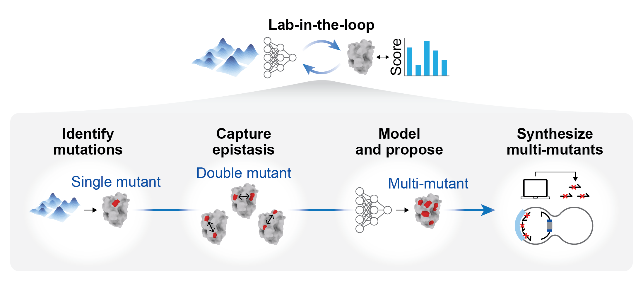
Workflow:
This module uses multiple protein language models to predict the potential effects of single-point mutations, enabling efficient screening of promising candidates for experimental validation. Four screening strategies are provided: ESM, ESM-IF, ESM-z, and ESM-IF-z. Residue indexing starts from 1.
ESM strategy, each ESM sub-model computes the conditional probability difference between the mutant amino acid and the wild-type amino acid at the target position under the wild-type sequence background. The log-probability difference is used as the raw score for each sub-model, and the final ESM score is obtained by averaging across all sub-models.ESM-IF strategy, structure information is incorporated. For each structure, a structural conditional score is computed for the mutation and wild type at the target position. The difference is used as the raw score. If multiple structures or conformations are provided, the final ESM-IF score is the average across all structures.ESM-z and ESM-IF-z apply z-score normalization to the corresponding raw scores, enabling better comparison and ranking across mutation sites.Note: Z-score refers to a standardization method. Two normalization strategies are supported and controlled by the Normalization parameter.
Input protein structure file in PDB or CIF format for structure-based scoring. Multiple conformations of the same structure are supported (compressed formats: .zip, .tar, .tar.gz, .tgz, .tar.bz2, .tbz2, .tar.xz, .txz). Scores are averaged across conformations to reduce bias from a single structure.
Specify chain IDs for single-point mutation recommendation. Multiple chains are separated by commas (e.g., A,B). If not specified, all chains in the structure will be analyzed.
Number of candidate single-point mutations recommended per chain for each integrated method. Default: 20.
Residues to exclude from mutation analysis. Format: Chain + residue index (starting from 1), e.g., A100. Multiple positions can be separated by commas and ranges are supported, e.g., A10-20,A25,B30-36,B40.
Defines the grouping strategy for z-score normalization. Options: aa_substitution_type (default) and aa_mutation.
aa_substitution_type: Groups mutations by substitution type (e.g., A→L, G→V). Focuses on “which amino acid is replaced by which”.aa_mutation: Groups mutations by the resulting amino acid. Focuses on “what amino acid it becomes”.Output CSV file name for single-point mutation results. Default: SP_Mutation.csv.
This module trains predictive models using experimental data to automatically screen and combine mutations, generating high-order mutation designs for experimental validation. A typical workflow involves generating experimental data from single- or double-point mutations, then training a model to predict higher-order combinations (≥3 sites).
Input protein structure file in PDB or CIF format.
Input .csv file containing the following required columns:
mutation: Mutation information in the format WildTypeResidue + Chain + Position + MutantResidue, e.g., KA100N. For multi-point mutations, use semicolons, e.g., GA48R;DB106A.property: Experimental fold-change (FC), defined as: mutant property / wild-type property.Note:
stderr.txt.Single-point mutation file used for combinatorial generation. Format:
TA192V
TB192K
AC167R
NA72A
Notes:
stderr.txt for errors.Number of top-ranked variants returned per mutation order. Default: 3 (e.g., top 3 for triple, quadruple, etc., up to decuple mutations).
Output CSV file name. Default: MP_Mutationcsv.
| Chain ID | Mutations | ESM | ESM-IF | ESM-z | ESM-IF-z | Count |
|---|---|---|---|---|---|---|
| A | F26L | 1 | 0 | 1 | 1 | 3 |
| A | A167R | 1 | 0 | 1 | 0 | 2 |
| … |
Field Description:
WildTypeResidue + Position + MutantResidue (index starts from 1), e.g., F26LEach method ranks candidates independently and selects top-N non-redundant mutations.
| Variant ID | Chain ID | Mutations Number | Mutations | Sequence | Average |
|---|---|---|---|---|---|
| 399 | A | 3 | N72A/A167R/T192K | … | 0.7711919 |
| … |
Field Description:
all file)/, between chains by ;:The output package MP_Mutation.tar.gz contains:
MP_Mutation.csvMP_Mutation_all.csv (complete results)
EpHod 是一个基于机器学习的酶最适 pH(pHopt)预测工具,旨在从氨基酸序列直接预测酶的最适工作 pH 值。
核心思想是通过蛋白质语言模型 ESM1v 提取酶序列特征,结合残差注意力机制(RLAT)和支持向量回归(SVR)进行集成预测。模型直接从序列数据中学习与 pHopt 相关的结构和生物物理特征,包括残基与催化中心的距离、溶剂分子可及性等。
输入的酶序列 FASTA 文件路径,必选项
FASTA 文件每条序列以 > 开头,格式示例:
>Q2YPV0 | Brucella abortus | 4.2.1.11 | 8.5 | 0.366
MTAIIDIVGREILDSRGNPTVEVDVVLEDGSFGRAAVPSGASTGAHEAVELRDGGSRYLGKGVEKAVEVVNGKIFDAIAGMDAESQLLIDQTLIDLDGSANKGNLGANAILGVSLAVAKAAAQASGLPLYRYVGGTNAHVLPVPMMNIINGGAHADNPIDFQEFMILPVGATSIREAVRYGSEVFHTLKKRLKDAGHNTNVGDEGGFAPNLKNAQAALDFIMESIEKAGFKPGEDIALGLDCAATEFFKDGNYVYEGERKTRDPKAQAKYLAKLASDYPIVTIEDGMAEDDWEGWKYLTDLIGNKCQLVGDDLFVTNSARLRDGIRLGVANSILVKVNQIGSLSETLDAVETAHKAGYTAVMSHRSGETEDSTIADLAVATNCGQIKTGSLARSDRTAYNQLIRIEEELGKQARYAGRSALKLL
输出预测结果文件名,默认为 prediction.csv
预测结果为 CSV 文件,包含以下列:
| 列名 | 说明 |
|---|---|
| index | 序列 ID |
| RLATtr | 基于注意力机制的预测酶最适 pH |
| SVR | 基于支持向量回归的预测酶最适 pH |
| Ensemble | 集成预测值(上述两者平均) |
EpHod is a machine learning tool for predicting enzyme optimum pH (pHopt) directly from amino acid sequences.
The core approach uses the protein language model ESM1v to extract enzyme sequence features, combined with Residual Light Attention (RLAT) and Support Vector Regression (SVR) for ensemble prediction. The model learns structural and biophysical features directly from sequence data that relate to pHopt, including residue proximity to catalytic centers and solvent accessibility.
Path to input enzyme sequence FASTA file, required
Each sequence in the FASTA file starts with >, example format:
>Q2YPV0 | Brucella abortus | 4.2.1.11 | 8.5 | 0.366
MTAIIDIVGREILDSRGNPTVEVDVVLEDGSFGRAAVPSGASTGAHEAVELRDGGSRYLGKGVEKAVEVVNGKIFDAIAGMDAESQLLIDQTLIDLDGSANKGNLGANAILGVSLAVAKAAAQASGLPLYRYVGGTNAHVLPVPMMNIINGGAHADNPIDFQEFMILPVGATSIREAVRYGSEVFHTLKKRLKDAGHNTNVGDEGGFAPNLKNAQAALDFIMESIEKAGFKPGEDIALGLDCAATEFFKDGNYVYEGERKTRDPKAQAKYLAKLASDYPIVTIEDGMAEDDWEGWKYLTDLIGNKCQLVGDDLFVTNSARLRDGIRLGVANSILVKVNQIGSLSETLDAVETAHKAGYTAVMSHRSGETEDSTIADLAVATNCGQIKTGSLARSDRTAYNQLIRIEEELGKQARYAGRSALKLL
Output prediction result filename, default prediction.csv
Prediction result is a CSV file with the following columns:
| Column | Description |
|---|---|
| index | Sequence ID |
| RLATtr | Attention-based pHopt prediction |
| SVR | Support vector regression prediction |
| Ensemble | Ensemble prediction (average of above) |

ESP (Enzyme-Substrate Prediction) 是一个用于预测酶-底物反应活性的机器学习工具,旨在为实验筛选提供优先级排序。
它要解决的问题是:在候选组合数量较大时,如何优先挑出更可能发生反应的酶-底物对,从而降低实验试错成本。
ESP 的核心思想是联合利用两类信息:
输入的底物-酶对列表文件,支持 .csv、.xlsx、.xls 格式,必选项
文件应包含两列:substrate 和 enzyme
substrate,enzyme
C00069,MARLPFYLLVISTLLLVVTADSFLARPPSSSFLHALSNKRASTPASLPSCSLDFLLQTRGGTAANAATTALPTSALVERKGGAAVALEGGKTLWEKSKVWVFIGLWYFFNVAFNIYNKKVLNALPLPWTVSIAQLGLGALYTMFLWLVRARKMPTIAAPEMKTLSILGVLHAVSHITAITSLGAGAVSFTHIVKSAEPFFSAVFAGLFFGQFFSLPVYAALIPVVSGVAYASLKELTFTWLSFWCAMASNVVCAARGVVVKGMMGGKPTQSKDLTSSNMYSVLTILAALVLLPFGALVEGPGLHAAWKAAAAHPSLTNGGTELAKYLVYSGLTFFLYNEVAFAALESLHPISHAVANTIKRVVIIVVSVLVFRNPMSTQSIIGSSTAVIGVLLYSLAKHYCK
底物列的列名,默认为 substrate
酶列的列名,默认为 enzyme
输出结果文件名,默认为 predictions.csv
输出的结果文件,CSV 格式,包含以下列:
| 列名 | 说明 |
|---|---|
| substrate | 底物 ID |
| enzyme | 酶的氨基酸序列 |
| complete | 数据是否完整(True/False) |
| metabolite_similarity_score | 代谢物与训练集的相似度分数 |
| metabolite in training set | 底物是否在训练集中 |
| #metabolite in training set | 训练集中相似代谢物数量 |
| Prediction | 预测值(0-1),值越高表示反应越可能发生 |
metabolite_similarity_score 反映底物与训练集的相似程度,可作为预测可信度的参考ESP (Enzyme-Substrate Prediction) is a machine learning tool for predicting enzyme-substrate reaction activity, designed to provide priority ranking for experimental screening.
It addresses the problem: when the number of candidate combinations is large, how to prioritize enzyme-substrate pairs that are more likely to react, thereby reducing experimental trial-and-error costs.
The core idea of ESP is to jointly utilize two types of information:
Input file containing substrate-enzyme pairs, supports .csv, .xlsx, .xls format, required
The file should contain two columns: substrate and enzyme
substrate,enzyme
C00069,MARLPFYLLVISTLLLVVTADSFLARPPSSSFLHALSNKRASTPASLPSCSLDFLLQTRGGTAANAATTALPTSALVERKGGAAVALEGGKTLWEKSKVWVFIGLWYFFNVAFNIYNKKVLNALPLPWTVSIAQLGLGALYTMFLWLVRARKMPTIAAPEMKTLSILGVLHAVSHITAITSLGAGAVSFTHIVKSAEPFFSAVFAGLFFGQFFSLPVYAALIPVVSGVAYASLKELTFTWLSFWCAMASNVVCAARGVVVKGMMGGKPTQSKDLTSSNMYSVLTILAALVLLPFGALVEGPGLHAAWKAAAAHPSLTNGGTELAKYLVYSGLTFFLYNEVAFAALESLHPISHAVANTIKRVVIIVVSVLVFRNPMSTQSIIGSSTAVIGVLLYSLAKHYCK
C00002,MKGRRRRRREYCKFALLLVLYTLVLLLVPSVLDGGRDGDKGAEHCPGLQRSLGVWSLEAAAAGEREQGAEARAAEEGGANQSPRFPSNLSGAVGEAVSREKQHIYVHATWRTGSSFLGELFNQHPDVFYLYEPMWHLWQALYPGDAESLQGALRDMLRSLFRCDFSVLRLYAPPGDPAARAPDTANLTTAALFRWRTNKVICSPPLCPGAPRARAEVGLVEDTACERSCPPVAIRALEAECRKYPVVVIKDVRLLDLGVLVPLLRDPGLNLKVVQLFRDPRAVHNSRLKSRQGLLRESIQVLRTRQRGDRFHRVLLAHGVGARPGGQSRALPAAPRADFFLTGALEVICEAWLRDLLFARGAPAWLRRRYLRLRYEDLVRQPRAQLRRLLRFSGLRALAALDAFALNMTRGAAYGADRPFHLSARDAREAVHAWRERLSREQVRQVEAACAPAMRLLAYPRSGEEGDAEQPREGETPLEMDADGAT
Column name for substrate, default substrate
Column name for enzyme, default enzyme
Output result filename, default predictions.csv
Output result file in CSV format, containing the following columns:
| Column | Description |
|---|---|
| substrate | Substrate ID |
| enzyme | Enzyme amino acid sequence |
| complete | Whether data is complete (True/False) |
| metabolite_similarity_score | Similarity score between metabolite and training set |
| metabolite in training set | Whether substrate is in training set |
| #metabolite in training set | Number of similar metabolites in training set |
| Prediction | Prediction score (0-1), higher values indicate higher reaction likelihood |
metabolite_similarity_score reflects the similarity between substrate and training set, which can be used as a reference for prediction reliabilityCatalytic Optimum Predictor (CatOpt) 是一个基于深度学习的酶催化剂特性预测工具,用于从蛋白质序列预测酶的最适 pH 、最适温度和热变性温度。
CatOpt 的核心思想是利用蛋白质语言模型 ESM2 提取酶序列的高维特征表征,结合多头自注意力机制的多尺度卷积神经网络,实现高精度的酶催化特性预测。
输入数据集路径,CSV格式
输入文件应包含 sequence 列,每行为蛋白质的氨基酸序列。
sequence
MARLPFYLLVISTLLLVVTADSFLARPPSSSFLHALSNKRASTPASLPSCSLDFLLQTRGGTAANAATTALPTSALVERKGGAAVALEGGKTLWEKSKVWVFIGLWYFFNVAFNIYNKKVLNALPLPWTVSIAQLGLGALYTMFLWLVRARKMPTIAAPEMKTLSILGVLHAVSHITAITSLGAGAVSFTHIVKSAEPFFSAVFAGLFFGQFFSLPVYAALIPVVSGVAYASLKELTFTWLSFWCAMASNVVCAARGVVVKGMMGGKPTQSKDLTSSNMYSVLTILAALVLLPFGALVEGPGLHAAWKAAAAHPSLTNGGTELAKYLVYSGLTFFLYNEVAFAALESLHPISHAVANTIKRVVIIVVSVLVFRNPMSTQSIIGSSTAVIGVLLYSLAKHYCK
MKGRRRRRREYCKFALLLVLYTLVLLLVPSVLDGGRDGDKGAEHCPGLQRSLGVWSLEAAAAGEREQGAEARAAEEGGANQSPRFPSNLSGAVGEAVSREKQHIYVHATWRTGSSFLGELFNQHPDVFYLYEPMWHLWQALYPGDAESLQGALRDMLRSLFRCDFSVLRLYAPPGDPAARAPDTANLTTAALFRWRTNKVICSPPLCPGAPRARAEVGLVEDTACERSCPPVAIRALEAECRKYPVVVIKDVRLLDLGVLVPLLRDPGLNLKVVQLFRDPRAVHNSRLKSRQGLLRESIQVLRTRQRGDRFHRVLLAHGVGARPGGQSRALPAAPRADFFLTGALEVICEAWLRDLLFARGAPAWLRRRYLRLRYEDLVRQPRAQLRRLLRFSGLRALAALDAFALNMTRGAAYGADRPFHLSARDAREAVHAWRERLSREQVRQVEAACAPAMRLLAYPRSGEEGDAEQPREGETPLEMDADGAT
预测任务类型:pHopt(最适 pH)、topt(最适温度)、tm(热变性温度)
输出结果文件路径,默认为prediction_results.csv
CSV 格式,包含以下列:
| 列名 | 说明 |
|---|---|
| id | 样本索引 |
| sequence | 蛋白质氨基酸序列 |
| pred_{task} | 预测值(pHopt/topt/tm) |
| 任务 | 预测值范围 |
|---|---|
| pHopt | 0 - 14 |
| topt | 0 - 120 °C |
| tm | 0 - 100 °C |
CatOpt is a deep learning-based tool for predicting enzyme catalytic properties, including optimal pH, optimal temperature, and melting temperature from protein sequences.
The core idea of CatOpt is to leverage the ESM2 protein language model to extract high-dimensional sequence features, combined with a multi-scale convolutional neural network with multi-head self-attention mechanism, achieving high-precision enzyme catalytic property prediction.
Path to the input dataset in CSV format.
The input file must contain a sequence column, with each row representing a protein amino acid sequence.
sequence
MARLPFYLLVISTLLLVVTADSFLARPPSSSFLHALSNKRASTPASLPSCSLDFLLQTRGGTAANAATTALPTSALVERKGGAAVALEGGKTLWEKSKVWVFIGLWYFFNVAFNIYNKKVLNALPLPWTVSIAQLGLGALYTMFLWLVRARKMPTIAAPEMKTLSILGVLHAVSHITAITSLGAGAVSFTHIVKSAEPFFSAVFAGLFFGQFFSLPVYAALIPVVSGVAYASLKELTFTWLSFWCAMASNVVCAARGVVVKGMMGGKPTQSKDLTSSNMYSVLTILAALVLLPFGALVEGPGLHAAWKAAAAHPSLTNGGTELAKYLVYSGLTFFLYNEVAFAALESLHPISHAVANTIKRVVIIVVSVLVFRNPMSTQSIIGSSTAVIGVLLYSLAKHYCK
MKGRRRRRREYCKFALLLVLYTLVLLLVPSVLDGGRDGDKGAEHCPGLQRSLGVWSLEAAAAGEREQGAEARAAEEGGANQSPRFPSNLSGAVGEAVSREKQHIYVHATWRTGSSFLGELFNQHPDVFYLYEPMWHLWQALYPGDAESLQGALRDMLRSLFRCDFSVLRLYAPPGDPAARAPDTANLTTAALFRWRTNKVICSPPLCPGAPRARAEVGLVEDTACERSCPPVAIRALEAECRKYPVVVIKDVRLLDLGVLVPLLRDPGLNLKVVQLFRDPRAVHNSRLKSRQGLLRESIQVLRTRQRGDRFHRVLLAHGVGARPGGQSRALPAAPRADFFLTGALEVICEAWLRDLLFARGAPAWLRRRYLRLRYEDLVRQPRAQLRRLLRFSGLRALAALDAFALNMTRGAAYGADRPFHLSARDAREAVHAWRERLSREQVRQVEAACAPAMRLLAYPRSGEEGDAEQPREGETPLEMDADGAT
Prediction task type: pHopt (optimal pH), topt (optimal temperature), tm (melting temperature)
Path to the output results file. Default: prediction_results.csv
CSV format with the following columns:
| Column | Description |
|---|---|
| id | Sample index |
| sequence | Protein amino acid sequence |
| pred_{task} | Prediction value (pHopt/topt/tm) |
| Task | Prediction Range |
|---|---|
| pHopt | 0 - 14 |
| topt | 0 - 120 °C |
| tm | 0 - 100 °C |

对结构预测模型(如:Boltz2/Protenix/AF3等)预测的一组蛋白单体或复合物结构进行全面分析,包括:二级结构、溶剂可及性、疏水性、残基接触、结构置信度等等,对分析结果进行统一整理和对比展示。
核心思路:以参考链为分析目标,将二级结构、溶剂可及性、疏水性、残基接触、模型置信度,以及可选的同源序列和保守性信息等等汇总到同一份报告中。
模块工作流 :
相互作用类型判断的阈值:
| 相互作用类型 | 相互作用表示的编号 | 对应阈值 |
|---|---|---|
| 疏水接触 | hp |
原子间距 < RvdW(A)+RvdW(B)+0.5 Å。 |
| 盐桥 | sb |
距离 < 4.0 Å。 |
| π-阳离子 | pc |
距离 < 6.0 Å,角度 < 60°。 |
| π-π 堆积 | ps |
中心距 < 7.0 Å,法向角 < 30°;ψ角 < 45°。 |
| T-stacking | ts |
中心距 < 5.0 Å,相对 90° 的法向偏差 < 30°;ψ角 < 45°。 |
| 范德华接触 | vdw |
原子间距 < RvdW(A)+RvdW(B)+0.5 Å。 |
| 直接氢键 | hbbb / hbsb / hbss / hblb / hbls / hbll |
D–A 距离 < 3.5 Å,静态结构默认角度阈值 180°。 |
| 水桥氢键 | wb / lwb |
每一段氢键距离< 3.5 Å,角度 > 110°。 |
| 扩展水桥氢键 | wb2 / lwb2 |
每一段氢键距离< 3.5 Å,角度> 110°。 |
输入蛋白结构,允许单个以及批量输出。单结构输入,支持 .pdb、.cif、.mmcif 结构格式批量输入需要以压缩包的形式,支持:.zip、.tar、.tar.gz、.tgz、.tar.bz2、.tbz2、.tar.xz、.txz,批量输入最大支持100个结构。
指定通过BLAST+搜索筛选的序列数据库。可选:SwissProt(UniProt知识库中的Swiss-Prot数据库)和 PDBAA(从实验确定的三维结构数据库PDB衍生的序列)。
指定BLAST+搜索识别序列匹配的保留阈值。E值表示给定序列比对的统计显著性。E值越低(越接近零),匹配的显著性越高,可选阈值:
1e-4、1e-5、1e-6、1e-7、1e-8、1e-9、1e-10、1e-11、1e-12。默认:1e-6
设置在序列搜索时,保留的最大序列数,可选数量:1~25。默认:5
指定一行序列展示的残基数量。默认:120
分析相互作用时,是否输出范德华相互作用,默认不输出。
输出protein_contacts_profile.html,内容展示如下:
注意: 若输入超过80个结构,HTML文档有可能过大而导致浏览器无法正常显示。

说明:
A. 摘要
在图的最上方,是当前活动面板的摘要区。
Reference Chain 表示当前正在查看的参考链;Residue Span 表示这条链在图中覆盖的残基范围;Model Count 表示本次一起参与比较的模型数量;Output Status 表示当前链面板的结果状态;Weak Contact Cutoff和Strong Contact CutoffHydropathy Window、E-value Threshold、Weak Contact Cutoff、Strong Contact Cutoff、Homolog Display Limit 和 Database 则对应这张图生成时使用的关键参数,说明如下:| 参数 | 默认值 | 说明 |
|---|---|---|
Hydropathy Window |
3 |
疏水性平滑窗口大小,用于计算 Kyte-Doolittle hydropathy。值越大,曲线越平滑;值越小,越能反映局部波动。应为正整数。 |
E-value Threshold |
1e-6 |
表示指定BLAST+搜索识别序列匹配的保留阈值E-value,E值越低(越接近零),匹配的显著性越高。 |
Weak Contact Cutoff |
3.7 Å |
弱接触的距离上限,按非氢原子之间的最短距离判断。只有当最短距离 <= 3.7 Å 时,残基间才会被视为存在接触。通常表示“接触判定的外层阈值”。 |
Strong Contact Cutoff |
3.2 Å |
强接触的距离阈值,按非氢原子之间的最短距离判断。当最短距离 < 3.2 Å 时记为强接触;否则若仍在 weak cutoff 内,则记为弱接触。 |
Homolog Display Limit |
5 |
最多检索并展示多少条同源序列。取值范围为 0-25;设为 0 时会跳过 homolog search,只保留 query 序列本身。 |
Database |
SWISSPROT |
用于同源搜索的数据库,PDBAA和SWISSPROT。 |
B. 二级结构与置信度
在结构部分,每个模型都会用图形标出参考链上的二级结构单元。
Alpha Helix、3₁₀ Helix 和 Pi Helix 都用卷曲波浪线表示,颜色不同,分别对应 α 螺旋、3₁₀ 螺旋和 π 螺旋。Strand 用箭头表示,箭头方向反映链段方向。Alpha Turn 和 Beta Turn 则表示两类更短的紧转角区域,通常出现在连接不同二级结构的局部片段中。如果输入结构中带有逐残基置信度信息,结构轨道还会按 pLDDT 着色。
pLDDT >= 90,通常可以把这部分看作局部较可信的区域;70 <= pLDDT < 90,整体骨架往往已经比较可靠;50 <= pLDDT < 70,说明这一段需要更谨慎地解释;pLDDT < 50,这类区域往往更灵活,也更容易出现不稳定或低置信度的构象。把“结构形态”和“置信度颜色”结合起来看:如果某个螺旋或链段在不同模型里都出现,但颜色差异明显,就说明该局部形态可能存在不确定性。
C.如果当前参考链被识别为抗体样链,还会额外显示一条 Antibody Numbering 轨道,并在界面中提供 Kabat、IMGT、Chothia 三种编号方案切换。
CDR1、CDR2、CDR3 位置,帮助快速判断互补决定区落在序列的哪一段;如果序列并不像抗体可变区,或者当前环境无法完成抗体编号,这条轨道可能不会显示。
D. 序列与同源信息
在结构轨道下方,报告会显示参考链的序列轴。
Query Sequence 表示目标序列本身;Exact Match 表示该位置与查询序列完全一致;`Similar Substitution 表示氨基酸虽然不同,但仍属于较保守的替换。阅读时,它能帮助你区分“模型之间结构有差异,但序列背景本身很保守”和“这一段本来就在同源序列里变化较大”这两种情况。
E. Accessibility与Hydropathy
在序列信息下面,报告会显示两条理化性质轨道。
Accessibility 用来表示残基在结构表面的暴露程度。
对于结构分析,这条轨道适合用来判断一个位点更像是核心残基、表面残基,还是潜在的界面区域。
Hydropathy 则描述序列在局部窗口中的疏水或亲水倾向。
这条轨道结合
Accessibility轨道一起观察,能更好的判断某一段结构是否符合直觉:例如,一个明显暴露的区域如果同时又很疏水,就值得进一步留意它是否参与界面作用或是否处在特殊构象环境中。
F. 接触与符号
接触轨道用来描述参考链残基与其他链、配体或小分子的相互作用。
蛋白-蛋白接触使用字母显示,字母表示接触对方所在的链。颜色用于区分接触强度:
3.2 A;3.2 A 到 3.7 A 之间。除了链字母,轨道里还会出现一些专门的符号。
S 用来标记二硫键;绿色通常表示链内二硫键,青色表示链间二硫键;# 表示接触对方与当前位置具有相同的残基编号和残基类型,常见于对称相关的接触关系;符号对照表建议先看“有没有接触”,再看“接触对象是谁”,最后再结合结构轨道判断这些接触是否稳定、是否集中出现在同一个局部区域。
符号对照表:
| 符号 | 说明 |
|---|---|
A-Z / a-z |
与对应链发生蛋白-蛋白接触 |
S |
二硫键位置 |
# |
与同编号、同类型残基发生对应接触 |
* |
与核酸接触 |
+ |
与离子接触 |
: |
与卟啉样或相关大环配体接触 |
" |
与糖类配体接触 |
^ |
与其他小分子或杂项配体接触 |
G. 底部图例
分成三列:
Structure 主要解释螺旋、折叠链和转角这些结构符号以及抗体编号;Tracks 主要解释序列比对、可及性、疏水性和置信度颜色;Contacts 主要解释强弱接触、二硫键和各类配体符号。接触残基对的详细信息文件contact_details.csv,示例如下:
| Chain | Residue | Pos | Other_Chain | Other_Residue | Other_Pos | Structures | Distances | Distance_Avg | Interaction Types |
|---|---|---|---|---|---|---|---|---|---|
| A | Y | 34 | C | S | 32 | 1;2;3;4;5 | 3.34;3.32;3.00;3.31;3.39 | 3.27 | |
| A | H | 38 | B | D | 104 | 1;2;3;4;5 | 3.69;3.95;2.95;2.98;2.95 | 3.30 | sb |
| A | Q | 46 | B | Y | 95 | 1;2;3;4;5 | 3.57;3.71;3.41;3.46;3.48 | 3.53 | |
| A | R | 96 | C | E | 54 | 1;4;5 | 3.74;3.60;3.99 | 3.77 | sb |
| B | R | 99 | C | D | 55 | 2;3;4;5 | 3.74;2.77;2.82;2.84 | 3.04 | sb |
说明:
| 字段 | 说明 |
|---|---|
| Chain | 第一个残基所在链。 |
| Residue | 第一个残基类型。 |
| Pos | 第一个残基从1开始的顺序编号。 |
| Other_Chain | 形成接触的另一残基所在链。 |
| Other_Residue | 另一残基类型。 |
| Other_Pos | 另一残基从1开始的顺序编号。 |
| Structures | 存在该接触残基对的结构编号列表,结构编号从1开始按出现顺序(见HTML文档中结构名称的展示顺序,从上向下)编号,使用分号 ; 分隔。 |
| Distances | 各结构中该残基对的最小接触距离,顺序与 Structures 对应。 |
| Distance_Avg | 所有接触距离(Distances)的平均值。 |
| Interaction Types | 相互作用类型,使用分号 ; 分隔;未匹配时为空。 |
接触残基的详细信息文件contact_residue_details.csv,示例如下:
| Chain | Residue | Pos | SASA_Rel_Avg | All | … |
|---|---|---|---|---|---|
| A | E | 1 | 0.68 | 0.40 | … |
| A | S | 32 | 0.34 | 1.00 | … |
| A | Y | 34 | 0.04 | 1.00 | … |
| A | Q | 46 | 0.51 | 1.00 | … |
| A | Q | 93 | 0.09 | 0.60 | … |
| B | S | 7 | 0.21 | 0.40 | … |
说明:
| 字段 | 说明 |
|---|---|
| Chain | 残基所在链。 |
| Residue | 残基类型。 |
| Pos | 残基从1开始的顺序编号。 |
| SASA_Rel_Avg | 该残基在全部结构中的平均相对溶剂可及性,取值范围为 0.00 到 1.00。 |
| Domain(Kabat/IMGT/Chothia) | 如果是抗体链,会显示残基对应的CDR区域 |
| All / Cluster_n | 该残基在全部结构/聚类结构簇中的作为接触残基出现的频率,取值范围为 0.00 到 1.00。当前示例包含 All 列,数值为0.40,表示该残基在全部结构的40%中作为接触残基出现。若存在多个聚类结构簇,还会增加 Cluster_1、Cluster_2 等列。 |
接触残基汇总文件contact_consensus.csv,示例如下:
| Cluster Id | Structure Count | Cluster Center | Combine Count | Consensus Count | Combine Residue | Consensus Residue | Consensus Residue (Threshold) |
|---|---|---|---|---|---|---|---|
| All | 5 | proteinx_lig_rank_1 | 87 | 52 | A1;A31-34;A36;A38;A40;A42;A46-48;A50;A53-54;A57;A59;A91;A95-100;A102;B7-10;B1… | A32;A34;A36;A38;A40;A42;A47-48;A50;A53-54;A57;A91;A95-96;A98-100;B33;B35;B39;… | A32;A34;A36;A38;A40;A42;A46-48;A50;A53-54;A57;A59;A91;A95-100;A102;B30;B33;B3… |
说明:
| 字段 | 说明 |
|---|---|
| Cluster Id | 统计范围标识。All 表示基于全部结构的统计;若存在多个聚类结构簇,还会出现 Cluster_1、Cluster_2 等结构簇范围统计。 |
| Structure Count | 当前统计范围内参与汇总的结构数量。 |
| Cluster Center | 当前簇的中心结构 |
| Combine Count | 当前统计范围内,接触残基并集的数量。 |
| Consensus Count | 当前统计范围内,接触残基交集的数量。 |
| Combine Residue | 接触残基并集列表。残基编号使用从1开始的顺序编号,并保留链前缀;连续区间会压缩为 A31-34 这种格式。 |
| Consensus Residue | 接触残基交集列表,格式与 Combine Residue 相同。 |
| Consensus Residue (Threshold) | 达到统计范围内,结构数量百分比阈值的接触残基列表,格式与 Combine Residue 相同。默认阈值为 0.5,表示统计范围内50%的结构中出现的接触残基列表。 |
结构聚类信息tm_clusters.csv,示例如下:
| Structure | Cluster Id | Cluster Size | Cluster Center | Is Representative |
|---|---|---|---|---|
| chai-1_rank_1 | 1 | 5 | proteinx_lig_rank_1 | 0 |
| chai-1_rank_2 | 1 | 5 | proteinx_lig_rank_1 | 0 |
| proteinx_lig_rank_1 | 1 | 5 | proteinx_lig_rank_1 | 1 |
| proteinx_lig_rank_2 | 1 | 5 | proteinx_lig_rank_1 | 0 |
| proteinx_lig_rank_3 | 1 | 5 | proteinx_lig_rank_1 | 0 |
说明:
| 字段 | 说明 |
|---|---|
| Structure | 结构名称,不带后缀。 |
| Cluster Id | 聚类后,该结构所属的结构簇编号。 |
| Cluster Size | 该结构所在簇的成员数量。 |
| Cluster Center | 该结构所在簇的中心结构名。 |
| Is Representative | 是否为该簇的代表结构;1 表示是,0 表示否。 |
用于聚类的相似性分数(TM_score)矩阵tm_score_matrix.csv,示例如下:
| Structure | chai-1_rank_1 | chai-1_rank_2 | proteinx_lig_rank_1 | proteinx_lig_rank_2 | proteinx_lig_rank_3 |
|---|---|---|---|---|---|
| chai-1_rank_1 | 1.00 | 1.00 | 0.97 | 0.97 | 0.97 |
| chai-1_rank_2 | 1.00 | 1.00 | 0.98 | 0.98 | 0.98 |
| proteinx_lig_rank_1 | 0.97 | 0.98 | 1.00 | 1.00 | 1.00 |
| proteinx_lig_rank_2 | 0.97 | 0.98 | 1.00 | 1.00 | 1.00 |
| proteinx_lig_rank_3 | 0.97 | 0.98 | 1.00 | 1.00 | 1.00 |
复合物中所有可能相互作用的列表cross_structure_interaction.csv,示例如下:
| Chain | Residue | Pos | Other_Chain | Other_Residue | Other_Pos | Structures | Count | Interaction Types |
|---|---|---|---|---|---|---|---|---|
| B | R | 38 | B | E | 46 | 1;2;3;4;5 | 5 | sb |
| C | K | 105 | C | W | 2 | 1;2;3;4;5 | 5 | pc |
| C | F | 22 | C | F | 7 | 1;2;3;4;5 | 5 | ps |
| B | Y | 27 | B | Y | 32 | 1;2;3;4;5 | 5 | ts |
| B | R | 38 | D | ATP | 1 | 3;4;5 | 3 | pc |
说明:
| 字段 | 说明 |
|---|---|
| Chain | 第一个残基所在链。 |
| Residue | 第一个残基类型;或配体名称,如 LIG。 |
| Pos | 第一个残基从1开始的顺序编号。 |
| Other_Chain | 另一残基所在链。 |
| Other_Residue | 另一残基类型/配体名称 |
| Other_Pos | 另一残基从1开始的顺序编号。 |
| Structures | 存在该相互作用的结构编号列表,结构编号从1开始按出现顺序(见HTML文档中结构名称的展示顺序,从上向下)编号,使用分号 ; 分隔。 |
| Count | Structures 中结构编号的数量。 |
| Interaction Types | 该相互作用对,相互作用类型汇总,使用分号 ; 分隔。 |
输出protein_contacts_profile_results.tar.gz,会包含HTML、PDF、CSV文档。
Performs comprehensive analysis on a set of protein monomer or complex structures predicted by structure prediction models (e.g., Boltz2 / Protenix / AF3), including secondary structure, solvent accessibility, hydrophobicity, residue contacts, structural confidence, and more. Analysis results are organized and presented in a unified comparative view.
Core concept: Using the reference chain as the analysis target, the report aggregates secondary structure, solvent accessibility, hydrophobicity, residue contacts, model confidence, and optionally homologous sequences and conservation information into a single document.
Module workflow:
Interaction type thresholds:
| Interaction Type | Code | Threshold |
|---|---|---|
| Hydrophobic contact | hp |
Inter-atomic distance < RvdW(A)+RvdW(B)+0.5 Å |
| Salt bridge | sb |
Distance < 4.0 Å |
| π-Cation | pc |
Distance < 6.0 Å, angle < 60° |
| π-π Stacking | ps |
Centroid distance < 7.0 Å, normal angle < 30°; ψ angle < 45° |
| T-stacking | ts |
Centroid distance < 5.0 Å, normal deviation from 90° < 30°; ψ angle < 45° |
| van der Waals contact | vdw |
Inter-atomic distance < RvdW(A)+RvdW(B)+0.5 Å |
| Direct H-bond | hbbb / hbsb / hbss / hblb / hbls / hbll |
D–A distance < 3.5 Å; default angle threshold 180° for static structures |
| Water-bridged H-bond | wb / lwb |
Each H-bond segment distance < 3.5 Å, angle > 110° |
| Extended water-bridged H-bond | wb2 / lwb2 |
Each H-bond segment distance < 3.5 Å, angle > 110° |
Input protein structures, supporting both single and batch submission. Single-structure input supports .pdb, .cif, and .mmcif formats. Batch input must be provided as a compressed archive, supporting .zip, .tar, .tar.gz, .tgz, .tar.bz2, .tbz2, .tar.xz, .txz. Maximum 100 structures per batch.
Specifies the sequence database for BLAST+ search filtering. Options: SwissProt (from the UniProt Knowledgebase) and PDBAA (derived from experimentally determined 3D structures in PDB).
Specifies the retention threshold for BLAST+ sequence match significance. The E-value indicates the statistical significance of a given sequence alignment. A lower E-value (closer to zero) indicates higher significance. Available thresholds: 1e-4, 1e-5, 1e-6, 1e-7, 1e-8, 1e-9, 1e-10, 1e-11, 1e-12. Default: 1e-6
Sets the maximum number of sequences retained during sequence search. Range: 1–25. Default: 5
Specifies the number of residues displayed per line. Default: 120
Whether to output van der Waals interactions during interaction analysis. Default: false
Outputs protein_contacts_profile.html, displayed as follows:
Note: If more than 80 structures are input, the HTML document may become too large for browsers to display properly.
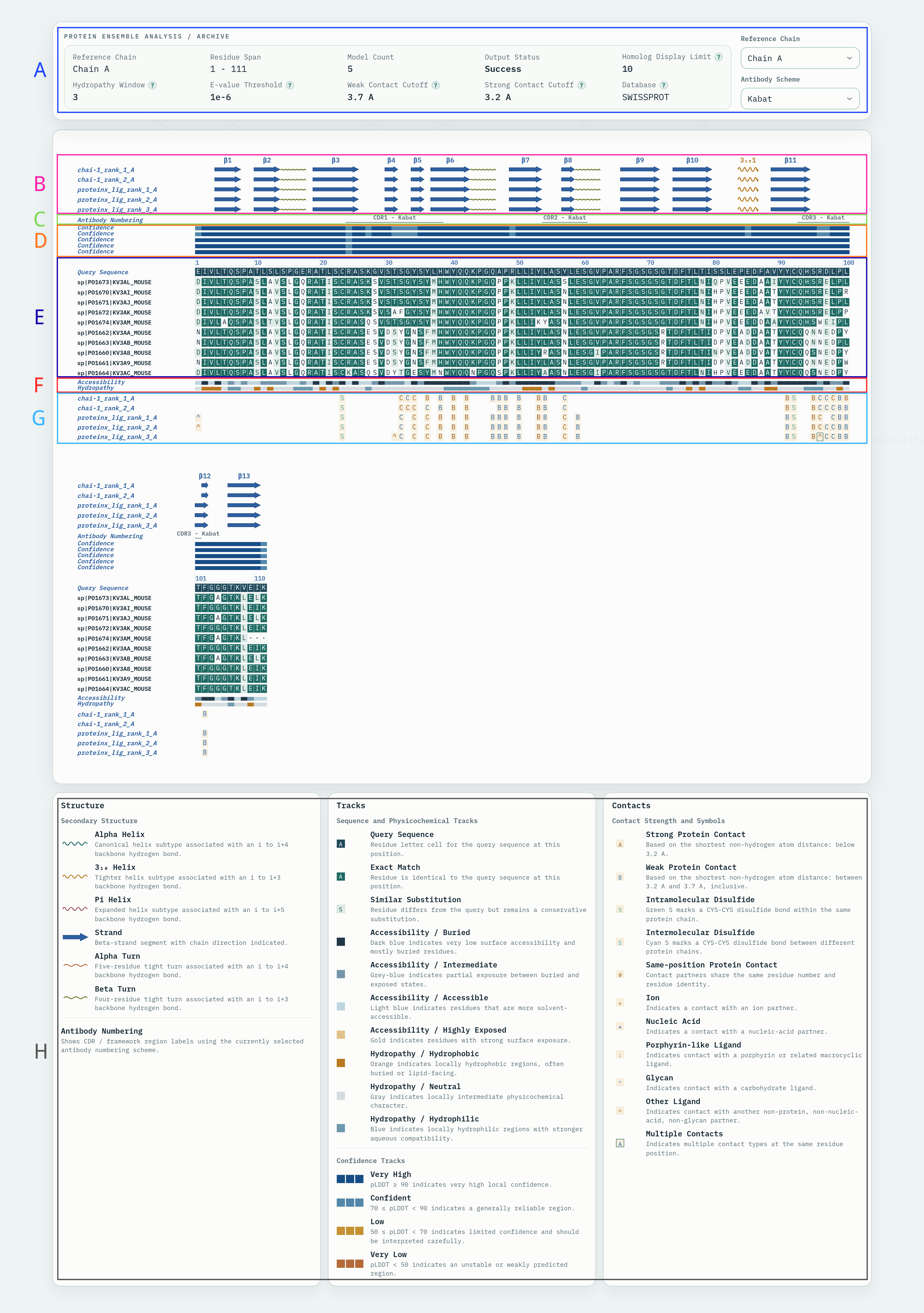
At the top of the figure is the summary area for the current active panel.
Reference Chain: the reference chain currently being viewed;Residue Span: the residue range covered by this chain in the figure;Model Count: the number of models participating in this comparison;Output Status: the result status of the current chain panel;Weak Contact Cutoff and Strong Contact CutoffHydropathy Window, E-value Threshold, Weak Contact Cutoff, Strong Contact Cutoff, Homolog Display Limit, and Database correspond to key parameters used during figure generation, described below:| Parameter | Default | Description |
|---|---|---|
Hydropathy Window |
3 |
Smoothing window size for Kyte-Doolittle hydropathy calculation. Larger values produce smoother curves; smaller values reflect local fluctuations more closely. Must be a positive integer. |
E-value Threshold |
1e-6 |
Retention threshold for BLAST+ sequence match significance. A lower E-value (closer to zero) indicates higher significance. |
Weak Contact Cutoff |
3.7 Å |
Upper distance limit for weak contacts, judged by the shortest distance between non-hydrogen atoms. A contact is only considered present when the shortest distance is <= 3.7 Å. This is typically the outer threshold for contact判定. |
Strong Contact Cutoff |
3.2 Å |
Distance threshold for strong contacts, judged by the shortest distance between non-hydrogen atoms. Distances < 3.2 Å are recorded as strong contacts; otherwise, if within the weak cutoff, they are recorded as weak contacts. |
Homolog Display Limit |
5 |
Maximum number of homologous sequences retrieved and displayed. Range: 0–25; setting to 0 skips homolog search and retains only the query sequence itself. |
Database |
SWISSPROT |
Database used for homology search: PDBAA or SWISSPROT. |
In the structure section, each model marks the secondary structure elements on the reference chain.
Alpha Helix, 3₁₀ Helix, and Pi Helix are all represented by coiled waves in different colors, corresponding to α-helix, 3₁₀-helix, and π-helix, respectively.Strand is represented by arrows, with arrow direction reflecting strand orientation.Alpha Turn and Beta Turn denote two classes of shorter tight-turn regions, typically appearing in local segments connecting different secondary structures.If the input structures contain per-residue confidence information, the structure tracks are colored by pLDDT.
pLDDT >= 90, typically regarded as locally highly reliable regions;70 <= pLDDT < 90, generally indicating a fairly reliable backbone;50 <= pLDDT < 70, suggesting this segment should be interpreted with caution;pLDDT < 50, regions that are often more flexible and prone to unstable or low-confidence conformations.Combining “structural morphology” with “confidence color”: if a helix or strand appears across multiple models but with noticeably different colors, it indicates potential uncertainty in the local conformation.
If the current reference chain is recognized as an antibody-like chain, an additional Antibody Numbering track is displayed, with toggle options for Kabat, IMGT, and Chothia numbering schemes in the interface.
CDR1, CDR2, and CDR3 in the antibody variable region, helping to quickly determine which sequence segment the complementarity-determining regions fall into;If the sequence does not resemble an antibody variable region, or if antibody numbering cannot be completed in the current environment, this track may not be displayed.
Below the structure tracks, the report displays the reference chain sequence axis.
Query Sequence: the target sequence itself;Exact Match: indicates complete identity with the query sequence at this position;Similar Substitution: indicates that the amino acid differs but belongs to a relatively conserved substitution.When reading, this helps distinguish between “structural differences across models but a highly conserved sequence background” and “this segment is inherently variable among homologous sequences.”
Below the sequence information, the report displays two physicochemical property tracks.
Accessibility indicates the degree of surface exposure of a residue in the structure.
For structural analysis, this track is useful for judging whether a site is more likely a core residue, a surface residue, or a potential interface region.
Hydropathy describes the hydrophobic or hydrophilic tendency of the sequence in a local window.
Observing this track together with the
Accessibilitytrack can better help determine whether a structural segment matches intuition: for example, a clearly exposed region that is also highly hydrophobic warrants further attention to whether it participates in interface interactions or resides in a special conformational environment.
Contact tracks describe interactions between reference chain residues and other chains, ligands, or small molecules.
Protein-protein contacts are displayed as letters indicating the chain of the contact partner. Colors distinguish contact strength:
< 3.2 Å;3.2 Å and 3.7 Å.In addition to chain letters, the track contains specialized symbols.
S marks disulfide bonds; green typically indicates intra-chain disulfide bonds, cyan indicates inter-chain disulfide bonds;# indicates that the contact partner shares the same residue number and residue type as the current position, commonly seen in symmetry-related contacts;Symbol Legend below.Recommended reading order: first check “whether there is a contact”, then “who the contact partner is”, and finally combine with structural tracks to judge whether these contacts are stable and whether they are concentrated in the same local region.
Symbol Legend:
| Symbol | Description |
|---|---|
A–Z / a–z |
Protein-protein contact with the corresponding chain |
S |
Disulfide bond position |
# |
Contact with a residue of the same number and same type |
* |
Contact with nucleic acid |
+ |
Contact with ion |
: |
Contact with porphyrin-like or related macrocyclic ligand |
" |
Contact with carbohydrate ligand |
^ |
Contact with other small molecule or miscellaneous ligand |
Divided into three columns:
Structure: mainly explains structural symbols for helices, strands, and turns, as well as antibody numbering;Tracks: mainly explains sequence alignment, accessibility, hydrophobicity, and confidence colors;Contacts: mainly explains strong/weak contacts, disulfide bonds, and various ligand symbols.File: contact_details.csv
Example:
| Chain | Residue | Pos | Other_Chain | Other_Residue | Other_Pos | Structures | Distances | Distance_Avg | Interaction Types |
|---|---|---|---|---|---|---|---|---|---|
| A | Y | 34 | C | S | 32 | 1;2;3;4;5 | 3.34;3.32;3.00;3.31;3.39 | 3.27 | |
| A | H | 38 | B | D | 104 | 1;2;3;4;5 | 3.69;3.95;2.95;2.98;2.95 | 3.30 | sb |
| A | Q | 46 | B | Y | 95 | 1;2;3;4;5 | 3.57;3.71;3.41;3.46;3.48 | 3.53 | |
| A | R | 96 | C | E | 54 | 1;4;5 | 3.74;3.60;3.99 | 3.77 | sb |
| B | R | 99 | C | D | 55 | 2;3;4;5 | 3.74;2.77;2.82;2.84 | 3.04 | sb |
Field descriptions:
| Field | Description |
|---|---|
| Chain | Chain of the first residue. |
| Residue | Type of the first residue. |
| Pos | Sequential 1-based index of the first residue. |
| Other_Chain | Chain of the contacting partner residue. |
| Other_Residue | Type of the partner residue. |
| Other_Pos | Sequential 1-based index of the partner residue. |
| Structures | List of structure indices where this contact pair exists. Structure indices start from 1 in order of appearance (see structure name display order in the HTML document, top to bottom), separated by semicolons ;. |
| Distances | Minimum contact distances for this residue pair in each structure, in the same order as Structures. |
| Distance_Avg | Average of all contact distances (Distances). |
| Interaction Types | Interaction type(s), separated by semicolons ;; empty if not matched. |
File: contact_residue_details.csv
Example:
| Chain | Residue | Pos | SASA_Rel_Avg | All | … |
|---|---|---|---|---|---|
| A | E | 1 | 0.68 | 0.40 | … |
| A | S | 32 | 0.34 | 1.00 | … |
| A | Y | 34 | 0.04 | 1.00 | … |
| A | Q | 46 | 0.51 | 1.00 | … |
| A | Q | 93 | 0.09 | 0.60 | … |
| B | S | 7 | 0.21 | 0.40 | … |
Field descriptions:
| Field | Description |
|---|---|
| Chain | Chain containing the residue. |
| Residue | Residue type. |
| Pos | Sequential 1-based index of the residue. |
| SASA_Rel_Avg | Average relative solvent-accessible surface area of this residue across all structures, ranging from 0.00 to 1.00. |
| Domain (Kabat/IMGT/Chothia) | If the chain is an antibody chain, displays the corresponding CDR region for the residue. |
| All / Cluster_n | Frequency with which this residue appears as a contact residue across all structures / within a structural cluster, ranging from 0.00 to 1.00. The example shows the All column with value 0.40, indicating this residue appeared as a contact residue in 40% of all structures. If multiple structural clusters exist, additional columns Cluster_1, Cluster_2, etc. will be added. |
File: contact_consensus.csv
Example:
| Cluster Id | Structure Count | Cluster Center | Combine Count | Consensus Count | Combine Residue | Consensus Residue | Consensus Residue (Threshold) |
|---|---|---|---|---|---|---|---|
| All | 5 | proteinx_lig_rank_1 | 87 | 52 | A1;A31-34;A36;A38;A40;A42;A46-48;A50;A53-54;A57;A59;A91;A95-100;A102;B7-10;B1… | A32;A34;A36;A38;A40;A42;A47-48;A50;A53-54;A57;A91;A95-96;A98-100;B33;B35;B39;… | A32;A34;A36;A38;A40;A42;A46-48;A50;A53-54;A57;A59;A91;A95-100;A102;B30;B33;B3… |
Field descriptions:
| Field | Description |
|---|---|
| Cluster Id | Statistical scope identifier. All indicates statistics based on all structures; if multiple structural clusters exist, additional scope statistics such as Cluster_1, Cluster_2, etc. will appear. |
| Structure Count | Number of structures included in the current statistical scope. |
| Cluster Center | Center structure of the current cluster. |
| Combine Count | Number of residues in the union of contact residues within the current statistical scope. |
| Consensus Count | Number of residues in the intersection of contact residues within the current statistical scope. |
| Combine Residue | List of contact residues in the union. Residue numbering uses 1-based sequential indexing with chain prefixes; contiguous ranges are compressed into formats such as A31-34. |
| Consensus Residue | List of contact residues in the intersection, formatted the same as Combine Residue. |
| Consensus Residue (Threshold) | List of contact residues reaching the percentage threshold of structures within the statistical scope, formatted the same as Combine Residue. Default threshold is 0.5, indicating contact residues that appeared in 50% of structures within the scope. |
File: tm_clusters.csv
Example:
| Structure | Cluster Id | Cluster Size | Cluster Center | Is Representative |
|---|---|---|---|---|
| chai-1_rank_1 | 1 | 5 | proteinx_lig_rank_1 | 0 |
| chai-1_rank_2 | 1 | 5 | proteinx_lig_rank_1 | 0 |
| proteinx_lig_rank_1 | 1 | 5 | proteinx_lig_rank_1 | 1 |
| proteinx_lig_rank_2 | 1 | 5 | proteinx_lig_rank_1 | 0 |
| proteinx_lig_rank_3 | 1 | 5 | proteinx_lig_rank_1 | 0 |
Field descriptions:
| Field | Description |
|---|---|
| Structure | Structure name, without file extension. |
| Cluster Id | Cluster index to which the structure belongs after clustering. |
| Cluster Size | Number of members in the cluster containing this structure. |
| Cluster Center | Center structure name of the cluster containing this structure. |
| Is Representative | Whether this structure is the representative of its cluster; 1 = yes, 0 = no. |
Similarity score (TM-score) matrix used for clustering: tm_score_matrix.csv
Example:
| Structure | chai-1_rank_1 | chai-1_rank_2 | proteinx_lig_rank_1 | proteinx_lig_rank_2 | proteinx_lig_rank_3 |
|---|---|---|---|---|---|
| chai-1_rank_1 | 1.00 | 1.00 | 0.97 | 0.97 | 0.97 |
| chai-1_rank_2 | 1.00 | 1.00 | 0.98 | 0.98 | 0.98 |
| proteinx_lig_rank_1 | 0.97 | 0.98 | 1.00 | 1.00 | 1.00 |
| proteinx_lig_rank_2 | 0.97 | 0.98 | 1.00 | 1.00 | 1.00 |
| proteinx_lig_rank_3 | 0.97 | 0.98 | 1.00 | 1.00 | 1.00 |
File: cross_structure_interaction.csv
Example:
| Chain | Residue | Pos | Other_Chain | Other_Residue | Other_Pos | Structures | Count | Interaction Types |
|---|---|---|---|---|---|---|---|---|
| B | R | 38 | B | E | 46 | 1;2;3;4;5 | 5 | sb |
| C | K | 105 | C | W | 2 | 1;2;3;4;5 | 5 | pc |
| C | F | 22 | C | F | 7 | 1;2;3;4;5 | 5 | ps |
| B | Y | 27 | B | Y | 32 | 1;2;3;4;5 | 5 | ts |
| B | R | 38 | D | ATP | 1 | 3;4;5 | 3 | pc |
Field descriptions:
| Field | Description |
|---|---|
| Chain | Chain of the first residue. |
| Residue | Type of the first residue; or ligand name, e.g. LIG. |
| Pos | Sequential 1-based index of the first residue. |
| Other_Chain | Chain of the partner residue. |
| Other_Residue | Type / ligand name of the partner residue. |
| Other_Pos | Sequential 1-based index of the partner residue. |
| Structures | List of structure indices where this interaction exists. Structure indices start from 1 in order of appearance (see structure name display order in the HTML document, top to bottom), separated by semicolons ;. |
| Count | Number of structure indices in Structures. |
| Interaction Types | Summary of interaction type(s) for this interaction pair, separated by semicolons ;. |
The output protein_contacts_profile_results.tar.gz contains HTML, PDF, and CSV documents.
.png)
模块能够计算出动力学轨迹体系的总偶极矩以及其波动情况。通过这些数据,可以计算出例如低介电常数介质的介电常数。对于具有净电荷的分子,其净电荷会在分子质心处进行扣除。
MD模拟后得到的路径文件,可以在GMX MD Run (GMX2024)模块或者AlphaAutoMD (GMX2024)模块中获取。
选择需要计算的结构组别:Backbone,Protein,DNA,RNA,Complex。
可以根据PDB中小分子的名称填写组别名称。
注意:其中Complex指的是蛋白-小分子复合物体系。
自定义需要计算的残基编号,连续参数可用“-”表示,不连续残基用逗号隔开,例如:1-10,15。
注意:
1.使用该参数时必须指定完整分子的残基范围,不允许截断结构或遗漏残基。
2.残基编号参考system.gro文件
自定义需要计算的原子编号,连续参数可用“-”表示,不连续残基用逗号隔开,例如:1-10,15。
注意:
1.使用该参数时必须指定完整分子的残基范围,不允许截断结构或遗漏残基。
2.原子编号参考system.gro文件
每一帧的间隔时间(单位ns)
输出结果包括:
| 输出文件名称 | 说明 |
|---|---|
| aver.csv | 偶极矩统计量的时间平均结果(CSV 格式) |
| aver.png | 偶极矩统计量随时间变化的可视化图像(PNG 格式) |
| Mtot.csv | 体系总偶极矩及其分量的时间序列数据(CSV 格式) |
| Mtot.png | 体系总偶极矩模长随时间变化的可视化图像(PNG 格式) |
其中aver.csv包括信息如下:
| 字段名称 | 说明 |
|---|---|
| Time (ns) | 模拟时间(单位:纳秒) |
| <|M|^2> | 体系总偶极矩模长平方的系综平均值 |
| <|M|>^2 | 体系总偶极矩模长系综平均值的平方 |
| <|M|^2> - <|M|>^2 | 总偶极矩模长的涨落项,表示偶极矩的方差 |
| <|M|>^2 / <|M|^2> | 归一化的偶极矩相关比值,可用于介电常数计算 |
其中Mtot.csv包括信息如下:
| 字段名称 | 说明 |
|---|---|
| Time (ns) | 模拟时间(单位:纳秒) |
| M_x | 体系总偶极矩在 x 方向的分量 |
| M_y | 体系总偶极矩在 y 方向的分量 |
| M_z | 体系总偶极矩在 z 方向的分量 |
| |M_tot| | 体系总偶极矩向量的模长 |
This module calculates the total dipole moment of a molecular dynamics trajectory system and its fluctuations. Based on these data, properties such as the dielectric constant of low-dielectric media can be derived. For molecules with a net charge, the net charge is subtracted at the molecular center of mass before the dipole moment calculation.
The trajectory file obtained after MD simulations. It can be generated by the GMX MD Run (GMX2024) module or the AlphaAutoMD (GMX2024) module.
Select the structural group to be included in the calculation: Backbone, Protein, DNA, RNA, or Complex.
Custom group names can also be specified based on the names of small molecules defined in the PDB file.
Note: Complex refers to a protein–small-molecule complex system.
Specify custom residue indices for calculation. Continuous ranges can be denoted using “-”, and non-contiguous residues should be separated by commas, e.g., 1-10,15.
Note:
system.gro file.Specify custom atom indices for calculation. Continuous ranges can be denoted using “-”, and non-contiguous atoms should be separated by commas, e.g., 1-10,15.
Note:
system.gro file.Time interval between successive frames used in the calculation (unit: nanoseconds).
The output results include the following files:
| Output file name | Description |
|---|---|
aver.csv |
Time-averaged dipole moment statistics (CSV format) |
aver.png |
Visualization of dipole moment statistics as a function of time (PNG format) |
Mtot.csv |
Time series data of the total dipole moment and its vector components (CSV format) |
Mtot.png |
Visualization of the magnitude of the total dipole moment over time (PNG format) |
aver.csv File Contents
| Field name | Description |
|---|---|
Time (ns) |
Simulation time (nanoseconds) |
<|M|^2> |
Ensemble average of the squared magnitude of the total dipole moment |
<|M|>^2 |
Square of the ensemble-averaged magnitude of the total dipole moment |
<|M|^2> - <|M|>^2 |
Fluctuation term of the dipole moment magnitude, representing its variance |
<|M|>^2 / <|M|^2> |
Normalized dipole correlation ratio, used for dielectric constant calculations |
Mtot.csv File Contents
| Field name | Description |
|---|---|
Time (ns) |
Simulation time (nanoseconds) |
M_x |
x-component of the total dipole moment |
M_y |
y-component of the total dipole moment |
M_z |
z-component of the total dipole moment |
|M_tot| |
Magnitude of the total dipole moment vector |
MMGBSA计算受体与配体之间的结合自由能,并且提供能量分解数据、结合常数(Ka)、抑制剂常数(Ki)。熵的计算采用的是张增辉教授的相互作用熵的方法,该方法直接从分子动力学模拟计算结合自由能的熵组分(相互作用熵或-TΔS),但是需要选取结构稳定部分进行计算。
本模块提供四种计算方法,其中 Trajectory 是针对进行分子动力学模拟轨迹后计算其受配体之间的结合自由能;One Structure 是针对一帧pdb结构或者对接得到的PDB结构计算受配体之间的结合自由能,MMGBSA of One Structure 计算流程中可以直接输入PDB进行计算。
Index Name 是输入受配体组别名称;Custom Name 则是输入受配体的在PDB中的残基编号。
MD模拟后得到的路径文件,可以在MD (GMX2024)模块或者AlphaAutoMD模块中获取。
受体名称,可以为Protein、DNA、RNA。
配体名称,可以为Protein、DNA、RNA。如果为小分子,填写其在PDB中的名称。如果体系中除了蛋白以外为配体(包括小分子)可用Other表示。
参考结构。默认system.gro。可以在GMX MD Run (GMX2024)模块的输出结果文件中找到。当周期性边界条件处理不当时可以使用该参数。
起始帧时间,单位ps。最好选取RMSD稳定时区进行计算,以消除结构不稳定时导致的整体熵偏大。
结束帧时间,单位ps。最好选取RMSD稳定时区进行计算,以消除结构不稳定时导致的整体熵偏大。
间隔时间,单位ps。
索引文件,ndx格式。当体系中存在膜结构的时候可以通过Membrane Solvation模块获取index.ndx文件。膜模拟中的受体为receptor,配体为ligand,膜为membrane。
定义受体组别进行结合能计算。组别中填写的为蛋白氨基酸或者核酸碱基的序号。例如1-213或者1-211,212-213。蛋白氨基酸或者核酸碱基序号从1开始重新编号,与初始pdb氨基酸编号无关。
定义配体组别进行结合能计算。组别中填写的为蛋白氨基酸或者核酸碱基的序号。例如1-213或者1-211,212-213。蛋白氨基酸或者核酸碱基序号从1开始重新编号,与初始pdb氨基酸编号无关。
拓扑文件,由MD Solvation模块或者Membrane Solvation模块得到。
结构文件,.gro格式,由MD Solvation模块或者Membrane Solvation模块得到。
体系参数压缩文件,tar.gz格式。由MD Solvation模块或者Membrane Solvation模块得到。
输出结果包括:
| 输出文件名称 | 说明 |
|---|---|
| MMGBSA_result.csv | MMGBSA结果汇总文件。 |
| MMGBSA_Residue.csv | 能量分解数据CSV文件。 |
| MMGBSA.pdb | 原子对应的MMGBSA能量放到PDB文件。可以做对应能量类别的表面图,从图的颜色深浅可以看出哪些区域对结合能贡献值较大。 |
| MMGBSA.tar.gz | MMGBSA所有原始文件。包括_mmgbsa_residue_#.txt是每个残基对应的每个能量类别的数值,共包含7个能量类别:范德华能(VDW)、静电能(ELE)、溶剂化能极性部分(PB)、溶剂化能非极性部分(SA)、VDW+ELE=MM、PB+SA=GBSA、MM+GBSA=Binding/MGBSA。_mmgbsa_residue.txt是对上述7个文件的总结,即为MMGBSA_Residue.csv对应的原始文件。_mmgbsa_atom#.pdb是将每个原子对应的能量类别放到pdb文件,与MMGBSA.pdb相似。 |
GROMACS: High performance molecular simulations through multi-level parallelism from laptops to supercomputers. M. J. Abraham, T. Murtola, R. Schulz, S. Páll, J. C. Smith, B. Hess, E. Lindahl, SoftwareX, 1, (2015), 19-25.
Duan L, Liu X, Zhang JZ. Interaction Entropy: A New Paradigm for Highly Efficient and Reliable Computation of Protein-Ligand Binding Free Energy. J Am Chem Soc. 2016 May 4;138(17):5722-8.
https://github.com/Electrostatics/apbs/blob/main/docs/index.rst
MMGBSA calculates the binding free energy between a receptor and a ligand, providing energy decomposition data, binding constants (Ka), and inhibitor constants (Ki). The entropy calculation uses the method of interaction entropy proposed by Professor Zhang Zenghui, which directly calculates the entropy component of the binding free energy (interaction entropy or -TΔS) from molecular dynamics simulations, but requires selecting stable structural regions for calculation. This module provides four calculation methods. Among them, Trajectory calculates the binding free energy between the receptor and ligand after molecular dynamics simulation trajectories; One Structure calculates the binding free energy between the receptor and ligand for a single frame PDB structure or a docked PDB structure; MMGBSA of One Structure allows direct input of a PDB for calculation. Index Name is the input receptor-ligand group name, while Custom Name is the input residue numbers of the receptor-ligand in the PDB.
Path file obtained after MD simulation, available in the MD (GMX2024) module or AlphaAutoMD module.
Name of the receptor, can be Protein, DNA, or RNA.
Name of the ligand, can be Protein, DNA, or RNA. If it is a small molecule, enter its name in the PDB. Use ‘Other’ if the system contains a ligand (including small molecules) other than proteins.
Reference structure. Default: system.gro.
This file can be found in the output results of the GMX MD Run (GMX2024) module.
Use this parameter when periodic boundary conditions are not handled properly.
Start frame time in ps. It is best to select a stable RMSD region for calculation to eliminate large overall entropy caused by structural instability.
End frame time in ps. It is best to select a stable RMSD region for calculation to eliminate large overall entropy caused by structural instability.
Time interval in ps.
Index file in ndx format. When there is a membrane structure in the system, you can obtain the index.ndx file through the Membrane Solvation module. In membrane simulations, the receptor is ‘receptor’, the ligand is ‘ligand’, and the membrane is ‘membrane’.
Define receptor groups for binding energy calculation. Enter the sequence numbers of protein amino acids or nucleic acid bases in the group. For example, 1-213 or 1-211,212-213. Protein amino acid or nucleic acid base numbers start from 1 and are independent of the initial pdb amino acid numbering.
Define ligand groups for binding energy calculation. Enter the sequence numbers of protein amino acids or nucleic acid bases in the group. For example, 1-213 or 1-211,212-213. Protein amino acid or nucleic acid base numbers start from 1 and are independent of the initial pdb amino acid numbering.
Topology file obtained from the MD Solvation module or Membrane Solvation module.
Structure file in .gro format obtained from the MD Solvation module or Membrane Solvation module.
System parameter compression file in tar.gz format. Obtained from the MD Solvation module or Membrane Solvation module.
The output includes:
| Output File Name | Description |
|---|---|
| MMGBSA_result.csv | Summary file of MMGBSA results. |
| MMGBSA_Residue.csv | Energy decomposition data in CSV format. |
| MMGBSA.pdb | MMGBSA energy corresponding to atoms in a PDB file. This can be used to create a surface map of energy categories, where the color depth indicates the regions contributing significantly to the binding energy. |
| MMGBSA.tar.gz | All original MMGBSA files. Includes mmgbsa_residue#.txt which contains the values of each energy category for each residue, totaling 7 energy categories: van der Waals energy (VDW), electrostatic energy (ELE), polar part of solvation energy (PB), nonpolar part of solvation energy (SA), VDW+ELE=MM, PB+SA=GBSA, MM+GBSA=Binding/MMGBSA. _mmgbsa_residue.txt is a summary of the above 7 files, corresponding to the original file MMGBSA_Residue.csv. _mmgbsa_atom#.pdb assigns the energy categories to each atom in a pdb file, similar to MMGBSA.pdb. |
GROMACS: High performance molecular simulations through multi-level parallelism from laptops to supercomputers. M. J. Abraham, T. Murtola, R. Schulz, S. Páll, J. C. Smith, B. Hess, E. Lindahl, SoftwareX, 1, (2015), 19-25.
Duan L, Liu X, Zhang JZ. Interaction Entropy: A New Paradigm for Highly Efficient and Reliable Computation of Protein-Ligand Binding Free Energy. J Am Chem Soc. 2016 May 4;138(17):5722-8.
https://github.com/Electrostatics/apbs/blob/main/docs/index.rst
Alanine Scan (MMGBSA)是计算丙氨酸突变后的结合自由能,并且提供能量分解数据、结合常数(Ka)、抑制剂常数(Ki)。熵的计算采用的是张增辉教授的相互作用熵的方法,该方法直接从分子动力学模拟计算结合自由能的熵组分(相互作用熵或-TΔS),但是需要选取结构稳定部分进行计算。
本模块提供四种计算方法,其中 Trajectory 是针对进行分子动力学模拟轨迹后计算其受配体之间的结合自由能;One Structure 是针对一帧pdb结构或者对接得到的PDB结构计算受配体之间的结合自由能,MMGBSA of One Structure 计算流程中可以直接输入PDB进行计算。
Index Name 是输入受配体组别名称;Custom Name 则是输入受配体的在PDB中的残基编号。
MD模拟后得到的路径文件,可以在MD (GMX2024)模块或者AlphaAutoMD模块中获取。
受体名称,可以为Protein、DNA、RNA。
配体名称,可以为Protein、DNA、RNA。如果为小分子,填写其在PDB中的名称。如果体系中除了蛋白以外为配体(包括小分子)可用Other表示。
参考结构。默认system.gro。可以在GMX MD Run (GMX2024)模块的输出结果文件中找到。当周期性边界条件处理不当时可以使用该参数。
突变扫描为丙氨酸(ALA)的氨基酸位置。格式为‘32-34,36’。蛋白氨基酸或者核酸碱基序号从1开始重新编号,与初始pdb氨基酸编号无关。
丙氨酸扫描时使用的力场。
起始帧时间,单位ps。最好选取RMSD稳定时区进行计算,以消除结构不稳定时导致的整体熵偏大。
结束帧时间,单位ps。最好选取RMSD稳定时区进行计算,以消除结构不稳定时导致的整体熵偏大。
间隔时间,单位ps。
索引文件,ndx格式。当体系中存在膜结构的时候可以通过Membrane Solvation模块获取index.ndx文件。膜模拟中的受体为receptor,配体为ligand,膜为membrane。只能是AMBER力场下构建的膜体系才能进行计算。
定义受体组别进行结合能计算。组别中填写的为蛋白氨基酸或者核酸碱基的序号。例如1-213或者1-211,212-213。蛋白氨基酸或者核酸碱基序号从1开始重新编号,与初始pdb氨基酸编号无关。
定义配体组别进行结合能计算。组别中填写的为蛋白氨基酸或者核酸碱基的序号。例如1-213或者1-211,212-213。蛋白氨基酸或者核酸碱基序号从1开始重新编号,与初始pdb氨基酸编号无关。
拓扑文件,由MD Solvation模块或者Membrane Solvation模块得到。
结构文件,.gro格式,由MD Solvation模块或者Membrane Solvation模块得到。
体系参数压缩文件,tar.gz格式。由MD Solvation模块或者Membrane Solvation模块得到。
输出结果包括:
| 输出文件名称 | 说明 |
|---|---|
| MMGBSA_result.csv/MMGBSA_Result_txt.tar.gz | 丙氨酸突变结果csv文件。 |
| MMGBSA_Residue.csv/MMGBSA_Residue_csv.tar.gz | 残基能量分解数据(CSV)。 |
| MMGBSA.pdb/MMGBSA_pdb.tar.gz | 突变后能量映射到 PDB 文件,可用于可视化结合能贡献区域。 |
| MMGBSA.tar.gz | 全部原始数据,包括: • _mmgbsa_residue_#.txt(7 类能量:VDW、ELE、PB、SA、MM、GBSA、Binding)• _mmgbsa_residue.txt(残基能量汇总,对应 MMGBSA_Residue.csv)• _mmgbsa_atom#.pdb(原子能量映射 PDB,类似 MMGBSA.pdb)。 |
| ALA_Scan_Results.csv | 丙氨酸扫描所有残基突变结果。 |
ALA_Scan_Results.csv,包含信息如下:
| 字段名称 | 说明 |
|---|---|
| index | 残基编号。 |
| Residue | 原始残基名称。 |
| Mutation Residue | 突变后的残基(通常为丙氨酸 ALA)。 |
| dH (kJ/mol) | 焓贡献。 |
| Tds (kJ/mol) | 熵贡献(TΔS)。 |
| dG (kJ/mol) | 结合自由能变化。决定结合强弱的关键指标。越负说明亲和力越强。 |
| Ki (µM/L) | 解离常数,结合亲和力的倒数。 |
| Ka (L/µM) | 结合常数,亲和力大小。 |
Ka 越大表示结合力强,Ki 越小表示抑制效果强。
GROMACS: High performance molecular simulations through multi-level parallelism from laptops to supercomputers. M. J. Abraham, T. Murtola, R. Schulz, S. Páll, J. C. Smith, B. Hess, E. Lindahl, SoftwareX, 1, (2015), 19-25.
Duan L, Liu X, Zhang JZ. Interaction Entropy: A New Paradigm for Highly Efficient and Reliable Computation of Protein-Ligand Binding Free Energy. J Am Chem Soc. 2016 May 4;138(17):5722-8.
https://github.com/Electrostatics/apbs/blob/main/docs/index.rst
Alanine Scan (MMGBSA) calculates the binding free energy after alanine mutations and provides energy decomposition data, binding constants (Ka), and inhibitor constants (Ki). The entropy calculation uses the method of interaction entropy proposed by Professor Zhang Zenghui, which directly calculates the entropy component of the binding free energy (interaction entropy or -TΔS) from molecular dynamics simulations, but requires selecting stable structural regions for calculation. This module provides four calculation methods. Among them, Trajectory calculates the binding free energy between the receptor and ligand after molecular dynamics simulation trajectories; One Structure calculates the binding free energy between the receptor and ligand for a single frame PDB structure or a docked PDB structure; MMGBSA of One Structure allows direct input of a PDB for calculation. Index Name is the input receptor-ligand group name, while Custom Name is the input residue numbers of the receptor-ligand in the PDB.
Path file obtained after MD simulation, available in the MD (GMX2024) module or AlphaAutoMD module.
Name of the receptor, can be Protein, DNA, or RNA.
Name of the ligand, can be Protein, DNA, or RNA. If it is a small molecule, enter its name in the PDB. Use ‘Other’ if the system contains a ligand (including small molecules) other than proteins.
Reference structure. Default: system.gro.
This file can be found in the output results of the GMX MD Run (GMX2024) module.
Use this parameter when periodic boundary conditions are not handled properly.
The mutation scans for the amino acid location of alanine (ALA). Must followed the format is ‘32-34,36’. The protein amino acid or nucleic acid number is re-numbered from 1, independent of the initial pdb amino acid number.
Force field used for alanine scanning.
Start frame time in ps. It is best to select a stable RMSD region for calculation to eliminate large overall entropy caused by structural instability.
End frame time in ps. It is best to select a stable RMSD region for calculation to eliminate large overall entropy caused by structural instability.
Time interval in ps.
Index file in ndx format. When there is a membrane structure in the system, you can obtain the index.ndx file through the Membrane Solvation module. In membrane simulations, the receptor is ‘receptor’, the ligand is ‘ligand’, and the membrane is ‘membrane’. Only membrane systems built under the AMBER force field can be calculated.
Define receptor groups for binding energy calculation. Enter the sequence numbers of protein amino acids or nucleic acid bases in the group. For example, 1-213 or 1-211,212-213. Protein amino acid or nucleic acid base numbers start from 1 and are independent of the initial pdb amino acid numbering.
Define ligand groups for binding energy calculation. Enter the sequence numbers of protein amino acids or nucleic acid bases in the group. For example, 1-213 or 1-211,212-213. Protein amino acid or nucleic acid base numbers start from 1 and are independent of the initial pdb amino acid numbering.
Topology file obtained from the MD Solvation module or Membrane Solvation module.
Structure file in .gro format obtained from the MD Solvation module or Membrane Solvation module.
System parameter compression file in tar.gz format. Obtained from the MD Solvation module or Membrane Solvation module.
The output includes:
| File Name | Description |
|---|---|
| MMGBSA_result.csv / MMGBSA_Result_txt.tar.gz | Alanine mutation result (csv file). |
| MMGBSA_Residue.csv / MMGBSA_Residue_csv.tar.gz | Residue energy decomposition data (CSV). |
| MMGBSA.pdb / MMGBSA_pdb.tar.gz | Energy mapped onto the PDB file after mutation, useful for visualizing binding energy contribution regions. |
| MMGBSA.tar.gz | Complete raw data, including: • _mmgbsa_residue_#.txt (7 energy terms: VDW, ELE, PB, SA, MM, GBSA, Binding) • _mmgbsa_residue.txt (residue energy summary, corresponding to MMGBSA_Residue.csv) • _mmgbsa_atom#.pdb (atomic energy mapped PDB files, similar to MMGBSA.pdb). |
| ALA_Scan_Results.csv | Results of alanine scanning mutations for all residues. |
| Field Name | Description |
|---|---|
| index | Residue index number. |
| Residue | Original residue name. |
| Mutation Residue | Mutated residue (typically alanine, ALA). |
| dH (kJ/mol) | Enthalpy change. |
| Tds (kJ/mol) | Entropy term (TΔS). |
| dG (kJ/mol) | Binding free energy change, the key indicator of binding strength. The more negative the value, the stronger the affinity. |
| Ki (µM/L) | Dissociation constant, reciprocal of binding affinity. |
| Ka (L/µM) | Association constant, magnitude of binding affinity. |
Larger Ka indicates stronger binding affinity, while smaller Ki indicates stronger inhibitory effect.
GROMACS: High performance molecular simulations through multi-level parallelism from laptops to supercomputers. M. J. Abraham, T. Murtola, R. Schulz, S. Páll, J. C. Smith, B. Hess, E. Lindahl, SoftwareX, 1, (2015), 19-25.
Duan L, Liu X, Zhang JZ. Interaction Entropy: A New Paradigm for Highly Efficient and Reliable Computation of Protein-Ligand Binding Free Energy. J Am Chem Soc. 2016 May 4;138(17):5722-8.
https://github.com/Electrostatics/apbs/blob/main/docs/index.rst

预测蛋白质序列中潜在的蛋白酶或化学试剂切割位点。模块基于PeptideCutter工具对应的文献资料复现。PeptideCutter 是瑞士生物信息学研究所(SIB)Expasy 平台提供的专业生物信息学工具。
支持的蛋白酶或化学试剂的切割规则如下:
| Enzyme / Chemical Name | Abbrev | P4 | P3 | P2 | P1 | P1’ | P2’ |
|---|---|---|---|---|---|---|---|
| Arg-C proteinase | ArgC | - | - | - | R | - | - |
| Asp-N endopeptidase | AspN | - | - | - | - | D | - |
| Asp-N endopeptidase + N-terminal Glu | AspN+AspGluN | - | - | - | - | D or E | - |
| BNPS-Skatole | BNPS | - | - | - | W | - | - |
| Caspase 1 | Casp1 | F,W,Y or L | - | H,A or T | D | not P,E,D,Q,K or R | - |
| Caspase 2 | Casp2 | D | V | A | D | not P,E,D,Q,K or R | - |
| Caspase 3 | Casp3 | D | M | Q | D | not P,E,D,Q,K or R | - |
| Caspase 4 | Casp4 | L | E | V | D | not P,E,D,Q,K or R | - |
| Caspase 5 | Casp5 | L or W | E | H | D | - | - |
| Caspase 6 | Casp6 | V | E | H or I | D | not P,E,D,Q,K or R | - |
| Caspase 7 | Casp7 | D | E | V | D | not P,E,D,Q,K or R | - |
| Caspase 8 | Casp8 | I or L | E | T | D | not P,E,D,Q,K or R | - |
| Caspase 9 | Casp9 | L | E | H | D | - | - |
| Caspase 10 | Casp10 | I | E | A | D | - | - |
| Chymotrypsin-high specificity (C-term to [FYW], not before P) | Ch_hi | - | - | - | F or Y | not P | - |
| - | - | - | W | not P | - | ||
| Chymotrypsin-low specificity (C-term to [FYWML], not before P) | Ch_lo | - | - | - | F,L or Y | not P | - |
| - | - | - | W | not M or P | - | ||
| - | - | - | M | not P or Y | - | ||
| - | - | - | H | not D,M,P or W | - | ||
| Clostripain (Clostridiopeptidase B) | Clost | - | - | - | R | - | - |
| CNBr | CNBr | - | - | - | M | - | - |
| Enterokinase | EK | D or E | D or E | D or E | K | - | - |
| Factor Xa | FXa | A,F,G,I,L,T,V or M | D or E | G | R | - | - |
| Formic acid | HCOOH | - | - | - | D | - | - |
| Glutamyl endopeptidase | GluC | - | - | - | E | - | - |
| GranzymeB | GzmB | I | E | P | D | - | - |
| Hydroxylamine (NH2OH) | Hydro | - | - | - | N | G | - |
| Iodosobenzoic acid | Iodo | - | - | - | W | - | - |
| LysC | LysC | - | - | - | K | - | - |
| LysN | LysN | - | - | - | - | K | - |
| Neutrophil elastase | Elast | - | - | - | A or V | - | - |
| NTCB (2-nitro-5-thiocyanobenzoic acid) | NTCB | - | - | - | - | C | - |
| Pepsin (pH1.3) | Pn1.3 | - | not H,K or R | not P | not R | F or L | not P |
| - | not H,K or R | not P | F or L | - | not P | ||
| Pepsin (pH>2) | Pn2p | - | not H,K or R | not P | not R | F,L,W or Y | not P |
| - | not H,K or R | not P | F,L,W or Y | - | not P | ||
| Proline-endopeptidase[*] | Prol | - | - | H,K or R | P | not P | - |
| Proteinase K | ProtK | - | - | - | A,E,F,I,L,T,V,W or Y | - | - |
| Staphylococcal peptidase I | Staph | - | - | not E | E | - | - |
| Tobacco etch virus protease | TEV | - | Y | - | Q | G or S | - |
| Thermolysin | Therm | - | - | - | not D or E | A,F,I,L,M or V | not P |
| Thrombin | Throm | - | - | G | R | G | - |
| A,F,G,I,L,T,V or M | A,F,G,I,L,T,V,W or R | P | R | not D or E | not D or E | ||
| Trypsin | Tryps | - | - | - | K or R | not P | - |
| - | - | W | K | not P | - | ||
| - | - | M | R | not P | - |
*注:脯氨酸内肽酶仅能切割序列不超过30个氨基酸的底物。一种特殊的β螺旋结构域调控蛋白质水解:参见 Fulop 等,1998 年。
Trypsin Exceptions (Blocking Rules)
| Enzyme Name | P4 | P3 | P2 | P1 | P1’ | P2’ |
|---|---|---|---|---|---|---|
| Trypsin | - | - | C or D | K | D | - |
| Trypsin | - | - | C | K | H or Y | - |
| Trypsin | - | - | C | R | K | - |
| Trypsin | - | - | R | R | H or R | - |
上传蛋白的序列文件,只能提交单链序列,FASTA格式
选择切割的切割酶或化学物质,输入all表示选择全部,同时支持多个输入,输入方式如:Tryps;Ch_hi(输出对应的缩写,使用;分隔)。仅限上方切割规则表中酶和化学物质。
输出All_in_One.csv,内容为输入序列中的切割点表,内容如下:
| Chain ID | Name of enzyme | No. of cleavages | Positions of cleavage sites |
|---|---|---|---|
| seq_1 | Arg-C proteinase | 1 | 14 |
| seq_1 | Asp-N endopeptidase | 1 | 2 |
| seq_1 | Asp-N endopeptidase + N-terminal Glu | 2 | 2, 6 |
| seq_1 | BNPS-Skatole | 1 | 4 |
| seq_1 | Chymotrypsin-high specificity (C-term to [FYW], not before P) | 1 | 4 |
| seq_1 | Chymotrypsin-low specificity (C-term to [FYWML], not before P) | 2 | 4, 6 |
| seq_1 | Clostripain (Clostridiopeptidase B) | 1 | 14 |
| seq_1 | Formic acid | 1 | 3 |
| seq_1 | Glutamyl endopeptidase | 1 | 7 |
| seq_1 | Iodosobenzoic acid | 1 | 4 |
| seq_1 | LysC | 1 | 1 |
| seq_1 | Neutrophil elastase | 1 | 13 |
| seq_1 | NTCB (2-nitro-5-thiocyanobenzoic acid) | 1 | 4 |
| seq_1 | Pepsin (pH>2) | 1 | 4 |
| seq_1 | Proteinase K | 5 | 2, 4, 7, 8, 13 |
| seq_1 | Staphylococcal peptidase I | 1 | 7 |
| seq_1 | Thermolysin | 2 | 1, 12 |
| seq_1 | Trypsin | 1 | 1 |
| seq_2 | Asp-N endopeptidase + N-terminal Glu | 3 | 2, 11, 17 |
| seq_2 | BNPS-Skatole | 2 | 2, 16 |
| seq_2 | Chymotrypsin-high specificity (C-term to [FYW], not before P) | 5 | 2, 5, 11, 16, 17 |
| seq_2 | Chymotrypsin-low specificity (C-term to [FYWML], not before P) | 9 | 1, 2, 5, 6, 9, 10, 11, 16, 17 |
| seq_2 | CNBr | 1 | 6 |
| seq_2 | Glutamyl endopeptidase | 3 | 3, 12, 18 |
| seq_2 | Iodosobenzoic acid | 2 | 2, 16 |
| seq_2 | LysC | 2 | 13, 15 |
| seq_2 | LysN | 2 | 12, 14 |
| seq_2 | Neutrophil elastase | 1 | 4 |
| seq_2 | NTCB (2-nitro-5-thiocyanobenzoic acid) | 1 | 13 |
| seq_2 | Pepsin (pH1.3) | 3 | 4, 5, 10 |
| seq_2 | Pepsin (pH>2) | 4 | 4, 5, 10, 16 |
| seq_2 | Proteinase K | 10 | 1, 2, 3, 4, 5, 11, 12, 16, 17, 18 |
| seq_2 | Staphylococcal peptidase I | 3 | 3, 12, 18 |
| seq_2 | Thermolysin | 3 | 4, 5, 10 |
| seq_2 | Trypsin | 2 | 13, 15 |
说明:
| 字段 | 说明 |
|---|---|
| Chain ID | 序列名称。 如果名称有重复时,会在原名称上添加上_dup1、如:A_dup1,1对应就是重复的次数。 |
| Name of enzyme | 蛋白酶/化学试剂名称,用于标识采用哪一种切割规则(例如 Arg-C proteinase、Asp-N endopeptidase、BNPS-Skatole、CNBr 等)。 |
| No. of cleavages | 该酶/试剂在对应序列上预测到的切割次数(切割位点数量)。应与 Positions of cleavage sites 中列出的位点个数一致。 |
| Positions of cleavage sites | 切割位点在序列中的位置编号列表。用逗号 + 空格分隔(例如 2, 4, 7)。酶或化学试剂的切割发生在序列对应位置之后。 |
输出All_in_One.html,内容将包含所有链的切割信息,展出如下:
All_in_One.html
输出clvg_site_pred_results.tar.gz,包含所有序列各自的csv以及HTML报告结果。
Predict potential protease or chemical reagent cleavage sites in protein sequences.
This module is reproduced based on the literature associated with the PeptideCutter tool.
PeptideCutter is a professional bioinformatics tool provided by the ExPASy platform of the Swiss Institute of Bioinformatics (SIB).
The supported protease and chemical reagent cleavage rules are listed below:
| Enzyme / Chemical Name | Abbrev | P4 | P3 | P2 | P1 | P1’ | P2’ |
|---|---|---|---|---|---|---|---|
| Arg-C proteinase | ArgC | - | - | - | R | - | - |
| Asp-N endopeptidase | AspN | - | - | - | - | D | - |
| Asp-N endopeptidase + N-terminal Glu | AspN+AspGluN | - | - | - | - | D or E | - |
| BNPS-Skatole | BNPS | - | - | - | W | - | - |
| Caspase 1 | Casp1 | F,W,Y or L | - | H,A or T | D | not P,E,D,Q,K or R | - |
| Caspase 2 | Casp2 | D | V | A | D | not P,E,D,Q,K or R | - |
| Caspase 3 | Casp3 | D | M | Q | D | not P,E,D,Q,K or R | - |
| Caspase 4 | Casp4 | L | E | V | D | not P,E,D,Q,K or R | - |
| Caspase 5 | Casp5 | L or W | E | H | D | - | - |
| Caspase 6 | Casp6 | V | E | H or I | D | not P,E,D,Q,K or R | - |
| Caspase 7 | Casp7 | D | E | V | D | not P,E,D,Q,K or R | - |
| Caspase 8 | Casp8 | I or L | E | T | D | not P,E,D,Q,K or R | - |
| Caspase 9 | Casp9 | L | E | H | D | - | - |
| Caspase 10 | Casp10 | I | E | A | D | - | - |
| Chymotrypsin-high specificity (C-term to [FYW], not before P) | Ch_hi | - | - | - | F or Y | not P | - |
| - | - | - | W | not P | - | ||
| Chymotrypsin-low specificity (C-term to [FYWML], not before P) | Ch_lo | - | - | - | F,L or Y | not P | - |
| - | - | - | W | not M or P | - | ||
| - | - | - | M | not P or Y | - | ||
| - | - | - | H | not D,M,P or W | - | ||
| Clostripain (Clostridiopeptidase B) | Clost | - | - | - | R | - | - |
| CNBr | CNBr | - | - | - | M | - | - |
| Enterokinase | EK | D or E | D or E | D or E | K | - | - |
| Factor Xa | FXa | A,F,G,I,L,T,V or M | D or E | G | R | - | - |
| Formic acid | HCOOH | - | - | - | D | - | - |
| Glutamyl endopeptidase | GluC | - | - | - | E | - | - |
| GranzymeB | GzmB | I | E | P | D | - | - |
| Hydroxylamine (NH2OH) | Hydro | - | - | - | N | G | - |
| Iodosobenzoic acid | Iodo | - | - | - | W | - | - |
| LysC | LysC | - | - | - | K | - | - |
| LysN | LysN | - | - | - | - | K | - |
| Neutrophil elastase | Elast | - | - | - | A or V | - | - |
| NTCB (2-nitro-5-thiocyanobenzoic acid) | NTCB | - | - | - | - | C | - |
| Pepsin (pH1.3) | Pn1.3 | - | not H,K or R | not P | not R | F or L | not P |
| - | not H,K or R | not P | F or L | - | not P | ||
| Pepsin (pH>2) | Pn2p | - | not H,K or R | not P | not R | F,L,W or Y | not P |
| - | not H,K or R | not P | F,L,W or Y | - | not P | ||
| Proline-endopeptidase[*] | Prol | - | - | H,K or R | P | not P | - |
| Proteinase K | ProtK | - | - | - | A,E,F,I,L,T,V,W or Y | - | - |
| Staphylococcal peptidase I | Staph | - | - | not E | E | - | - |
| Tobacco etch virus protease | TEV | - | Y | - | Q | G or S | - |
| Thermolysin | Therm | - | - | - | not D or E | A,F,I,L,M or V | not P |
| Thrombin | Throm | - | - | G | R | G | - |
| A,F,G,I,L,T,V or M | A,F,G,I,L,T,V,W or R | P | R | not D or E | not D or E | ||
| Trypsin | Tryps | - | - | - | K or R | not P | - |
| - | - | W | K | not P | - | ||
| - | - | M | R | not P | - |
*Note: Proline endopeptidase can only cleave substrates with sequences shorter than 30 amino acids.
A special β-propeller domain regulates protein hydrolysis. See Fulop et al., 1998.
| Enzyme Name | P4 | P3 | P2 | P1 | P1’ | P2’ |
|---|---|---|---|---|---|---|
| Trypsin | - | - | C or D | K | D | - |
| Trypsin | - | - | C | K | H or Y | - |
| Trypsin | - | - | C | R | K | - |
| Trypsin | - | - | R | R | H or R | - |
Upload the protein sequence file.
Only single-chain sequences are supported, and the file must be in FASTA format.
Select the protease or chemical reagent for cleavage.
Enter all to select all enzymes. Multiple inputs are supported.
Example:
Tryps;Ch_hi
The corresponding abbreviations will be used in the output and should be separated by ;.
Only enzymes and chemicals listed in the cleavage rule table above are allowed.
The output All_in_One.csv contains the predicted cleavage sites for the input sequences.
| Chain ID | Name of enzyme | No. of cleavages | Positions of cleavage sites |
|---|---|---|---|
| seq_1 | Arg-C proteinase | 1 | 14 |
| seq_1 | Asp-N endopeptidase | 1 | 2 |
| seq_1 | Asp-N endopeptidase + N-terminal Glu | 2 | 2, 6 |
| seq_1 | BNPS-Skatole | 1 | 4 |
| seq_1 | Chymotrypsin-high specificity (C-term to [FYW], not before P) | 1 | 4 |
| … | … | … | … |
(remaining rows unchanged)
| Field | Description |
|---|---|
| Chain ID | The sequence name. If duplicate names appear, a suffix such as _dup1 will be added (e.g., A_dup1), where 1 represents the duplication count. |
| Name of enzyme | The protease or chemical reagent used to identify the applied cleavage rule (e.g., Arg-C proteinase, Asp-N endopeptidase, BNPS-Skatole, CNBr). |
| No. of cleavages | The number of predicted cleavage events in the sequence for the given enzyme or reagent. This number should match the count of sites listed in Positions of cleavage sites. |
| Positions of cleavage sites | A list of cleavage site positions within the sequence. Values are separated by comma + space (e.g., 2, 4, 7). Cleavage occurs after the corresponding residue position. |
The output All_in_One.html contains the cleavage information for all chains.
The output clvg_site_pred_results.tar.gz contains individual CSV files and HTML reports for each sequence.
Humaness Score (BioPhi)是抗体序列人源化评分工具,不依赖于有限的人源种系(germline)序列,而是基于海量的天然人类抗体库(Observed Antibody Space, OAS)。该数据库包含来自数百个受试者的数亿条序列,这使得它能捕捉到更丰富、更多样化的抗体序列空间。将待评估的抗体序列切割成所有可能的、长度为9个氨基酸的短肽(9-mer),将这些短肽放到庞大的OAS数据库中进行搜索,找出每个短肽在真实人类抗体库中出现的频率,以及携带该短肽的个体数量。如果一个序列中的大多数短肽在人类抗体库中都很常见,那么它的OASis评分就高,意味着“看起来很人类”,免疫原性风险较低;反之,如果含有大量在人类中罕见的短肽,则评分低,提示可能需要进一步人源化改造。
抗体序列文件,FASTA格式,同一抗体轻重链序列名可以通过后缀.H/.L、_VH/_VL、_HC/_LC识别,如:
Antibody1.H
XXXX
Antibody1.L
XXXX
Antibody2.H
XXXX
Antibody2.L
XXXX
支持批量,最大支持1000条序列计算,超过1000的序列会忽略。
编号方案,可选值包括 kabat、chothia、imgt、aho,默认值为 kabat
CDR 定义方法,可选值包括 kabat、chothia、imgt、north,默认值为 kabat
考虑肽段为人类的最小 OAS 主体百分比,取值范围为 1-90,默认值为 10.0
输出序列人源化打分文件名称,XLSX格式
输出文件默认为humaness_score.xlsx,文件中包含多个SHEET,第一个Overview内容包括:
| 列名 | 说明 |
|---|---|
| Antibody | 抗体名称 |
| Threshold | 使用的阈值,loose:宽松 (≥1% subjects),relaxed 较宽松(≥10% subjects),medium 中等(≥50% subjects),strict 严格(≥90% subjects) |
| OASis Percentile | 抗体整体(重链+轻链)的 OASis 百分位数,得分越高,代表该序列在人类天然抗体库中出现的频率越高 |
| OASis Identity | 抗体序列与人类天然抗体库中最接近序列的同一性(相似度) |
| Germline Content | 重链+轻链的胚系含量(与人类最接近的 V/J 基因的整体相似度) |
| Heavy V Germline | 重链 V 基因来源 |
| Heavy J Germline | 重链 J 基因来源 |
| Heavy OASis Percentile | 重链的 OASis 百分位数 |
| Heavy OASis Identity | 重链与最接近人类胚系基因的相似度 |
| Heavy Non-human peptides | 重链检测到的非人源肽段的数量 |
| Heavy Germline Content | 重链的胚系含量(与人类最接近的 V/J 基因的整体相似度) |
| Light V Germline | 轻链 V 基因来源 |
| Light J Germline | 轻链 J 基因来源 |
| Light OASis Percentile | 轻链的 OASis 百分位数 |
| Light OASis Identity | 轻链与最接近人类胚系基因的相似度 |
| Light Non-human peptides | 轻链检测到的非人源肽段的数量 |
| Light Germline Content | 轻链的胚系含量(与人类最接近的 V/J 基因的整体相似度) |
Humaness Score (BioPhi) is a tool for evaluating the humanization score of antibody sequences. It does not rely on a limited set of human germline sequences but is instead based on the vast natural human antibody repertoire, the Observed Antibody Space (OAS). This database contains hundreds of millions of sequences from hundreds of subjects, allowing it to capture a richer, more diverse landscape of antibody sequences. The tool evaluates an antibody sequence by slicing it into all possible 9-amino-acid peptides (9-mers) and searching for these peptides within the extensive OAS database. It determines the frequency of each peptide in the authentic human antibody repertoire and the number of individuals carrying that peptide. If most peptides in a sequence are common in the human antibody repertoire, the sequence receives a high OASis score, indicating it “looks human” and has a lower risk of immunogenicity. Conversely, if the sequence contains many peptides that are rare in humans, the score is low, suggesting that further humanization may be needed.
Antibody sequence file in FASTA format. For the same antibody, heavy and light chain sequences can be identified using suffixes such as .H/.L, _VH/_VL, or _HC/_LC. Example:
Antibody1.H
XXXX
Antibody1.L
XXXX
Antibody2.H
XXXX
Antibody2.L
XXXX
Batch processing is supported, with a maximum of 1,000 sequences for calculation. Sequences exceeding 1,000 will be ignored.
Numbering scheme, options include kabat, chothia, imgt, aho, default value is kabat
CDR definition method, options include kabat, chothia, imgt, north, default value is kabat
Minimum percent of OAS subjects to consider peptide human, range 1-90, default value is 10.0
The name of the output file containing the humanization scores for the sequences, in XLSX format.
The default output file is humaness_score.xlsx, which contains multiple sheets. The first sheet, “Overview,” includes the following columns:
| Column | Description |
|---|---|
| Antibody | Antibody name |
| Threshold | Input threshold used, loose (≥1% subjects),relaxed (≥10% subjects),medium (≥50% subjects),strict (≥90% subjects) |
| OASis Percentile | Overall (heavy + light chain) OASis percentile of the antibody. A higher score indicates a higher frequency of the sequence in the natural human antibody repertoire. |
| OASis Identity | Overall identity (similarity) of the antibody sequence to the closest sequence in the natural human antibody repertoire. |
| Germline Content | Overall germline content (heavy + light chain) – the overall similarity to the closest human V/J genes. |
| Heavy V Germline | V gene origin for the heavy chain. |
| Heavy J Germline | J gene origin for the heavy chain. |
| Heavy OASis Percentile | OASis percentile for the heavy chain. |
| Heavy OASis Identity | Identity of the heavy chain to the closest human germline gene. |
| Heavy Non-human peptides | Number of non-human peptides detected in the heavy chain. |
| Heavy Germline Content | Germline content for the heavy chain – similarity to the closest human V/J genes. |
| Light V Germline | V gene origin for the light chain. |
| Light J Germline | J gene origin for the light chain. |
| Light OASis Percentile | OASis percentile for the light chain. |
| Light OASis Identity | Identity of the light chain to the closest human germline gene. |
| Light Non-human peptides | Number of non-human peptides detected in the light chain. |
| Light Germline Content | Germline content for the light chain – similarity to the closest human V/J genes. |

进行DNA序列比对(查询序列VS模板序列),分析序列突变(相对于模板序列),并给出翻译的氨基酸序列,及其对应的残基突变(相对于模板序列)。
DNA模板序列,fasta格式,支持多条。
DNA查询序列,fasta格式文件或.seq文本文件(每个文件单一序列),支持批量,以打包压缩文件上传即可。
比对结果文件名。默认:dna_analysis_res.csv
输出dna_analysis_res.csv,字段说明:
| 字段名 | 说明 |
|---|---|
query |
查询序列名称,取FASTA文件中的序列ID或.seq 文件名 |
target |
命中的模板序列名称,对应模板 FASTA 中的序列 ID |
template_nt_seq |
模板的对齐序列(命中区域),可能包含 gap(-) |
matched_nt_seq |
查询序列与模板对齐的部分(命中区域),可能包含 gap(-) |
identity |
序列一致性百分比,例如 99.300,单位 % |
template_aa_aln |
基于模板的对齐序列,翻译的氨基酸序列,可能包含 gap(-) |
matched_aa_aln |
基于查询序列的对齐序列,翻译的氨基酸序列,可能包含 gap(-) |
nt_mutations |
核酸突变列表(相对模板) |
aa_mutations |
氨基酸突变列表(相对模板) |
突变表示规则
| 表示格式 | 含义 |
|---|---|
A123G |
第 123 位由 A 替换为 G |
del123A |
删除模板第 123 位的 A |
ins123_T |
在模板第 123 位之后插入 T |
Perform DNA sequence comparison (Query Sequence VS Template Sequence), analyze sequence mutations (relative to the template sequence), and provide the translated amino acid sequences along with their corresponding residue mutations (relative to the template sequence).
DNA template sequences, FASTA format, supports multiple sequences.
DNA query sequences, FASTA format file or .seq text file (single sequence per file), supports batch processing, please upload as a compressed archive.
Alignment results filename. Default: dna_analysis_res.csv
Output dna_analysis_res.csv, field descriptions:
| Field Name | Description |
|---|---|
query |
Query sequence name, taken from the sequence ID in the FASTA file or the .seq filename |
target |
Matched template sequence name, corresponding to the sequence ID in the template FASTA |
template_nt_seq |
Aligned template sequence (hit region), may contain gaps (-) |
matched_nt_seq |
Part of the query sequence aligned with the template (hit region), may contain gaps (-) |
identity |
Sequence identity percentage, e.g., 99.300, unit % |
template_aa_aln |
Translated amino acid sequence based on the aligned template sequence, may contain gaps (-) |
matched_aa_aln |
Translated amino acid sequence based on the aligned query sequence, may contain gaps (-) |
nt_mutations |
List of nucleotide mutations (relative to the template) |
aa_mutations |
List of amino acid mutations (relative to the template) |
Mutation Representation Rules
| Representation Format | Meaning |
|---|---|
A123G |
Substitution of A with G at position 123 |
del123A |
Deletion of A at position 123 of the template |
ins123_T |
Insertion of T after position 123 of the template |
EZSpecificity 是用于酶-底物特异性预测的模型化工具,目标是为实验筛选提供优先级排序。
它要解决的问题是:在候选组合数量较大时,如何优先挑出更可能发生反应的酶-底物对,从而降低实验试错成本。
根据论文报告,EZSpecificity 在未知酶/未知底物等外推场景下,相比对照方法(如 ESP)表现更稳定,并在卤化酶案例中给出更高的 Top-1 命中率。
因此,它的定位是"实验前的筛选与排序工具",而不是"替代实验的最终判定工具"。
EZSpecificity 的核心思想是联合利用三类信息:
适用于大规模筛选场景,输入酶序列文件和底物列表,自动生成 N×N 组合进行预测。
酶的序列文件,FASTA格式,支持多条序列,必选项
>enzyme_405
MLPLQDFPKFTAAAVQASPVFLDAHKTAQKAVDLIAEAAGNGAELVVFPEVF...
>enzyme_483
MQTRKIVRAAAVQAASPNYDLATGVDKTIELARQARDEGCDLIVFGETWL...
底物分子的结构信息,支持.smi格式,必选项
substrate_smiles
N#CC1=NC=CC=C1 sample_1
N#CCC1=CC=CC=C1 sample_2
输出的结果文件, CSV 格式(默认文件名 predicted_scores.csv)
适用于使用复合物结构进行预测的场景,通过 CSV 文件指定底物与结构的对应关系。
输入的CSV文件,文件中需包含底物结构substrate_smiles 列和复合物结构名称complex_name 列,必选项
substrate_smiles,complex_name
N#CC1=NC=CC=C1,complex_405
N#CCC1=CC=CC=C1,complex_483
复合物结构压缩包,支持 .zip/.tar/.tar.gz/.tgz/.tar.bz2/.tar.xz 格式,必选项
压缩包内应包含与 complex_name 对应的 PDB 文件(如 complex_405.pdb)
输入的CSV文件中SMILES列的列名,必选项
输入的CSV文件中复合物名称列的列名,必选项
输出的结果文件, CSV 格式(默认文件名 predicted_scores.csv)
解析后记录错误的列表文件(如有),CSV格式(默认文件名match_errors.csv)
输出的结果文件, CSV 格式(默认文件名 predicted_scores.csv)
| 列名 | 说明 |
|---|---|
| substrate_smiles | 底物的 SMILES 字符串 |
| enzyme_sequence | 酶的氨基酸序列 |
| score | 预测打分值,数值越高表示该酶-底物对越可能发生反应 |
输出的结果文件, CSV 格式(默认文件名 predicted_scores.csv)
| 列名 | 说明 |
|---|---|
| substrate_smiles | 底物的 SMILES 字符串 |
| enzyme_sequence | 酶的氨基酸序列 |
| score | 预测打分值,数值越高表示该酶-底物对越可能发生反应 |
| complex_name | 复合物结构名称 |
| matched_complex_file | 根据复合物名称匹配到的结构文件 |
解析后记录错误的列表文件(如有),CSV格式(默认文件名match_errors.csv)
| 列名 | 说明 |
|---|---|
| complex_name | 匹配失败的复合物结构名称 |
| error | 匹配失败的原因或错误信息 |
EZSpecificity is a modeling tool for enzyme-substrate specificity prediction, designed to provide priority ranking for experimental screening.
It addresses the problem: when the number of candidate combinations is large, how to prioritize enzyme-substrate pairs that are more likely to react, thereby reducing experimental trial-and-error costs.
According to the paper, EZSpecificity demonstrates more stable performance compared to control methods (such as ESP) in extrapolation scenarios involving unknown enzymes/unknown substrates, and achieves higher Top-1 hit rates in halogenase case studies.
Therefore, its positioning is a “pre-experimental screening and ranking tool” rather than a “final decision tool to replace experiments”.
The core idea of EZSpecificity is to jointly utilize three types of information:
The final model outputs a score for ranking.
Suitable for large-scale screening scenarios. Input enzyme sequence files and substrate lists to automatically generate N×N combinations for prediction.
Enzyme sequence file in FASTA format, supporting multiple sequences. Required.
>enzyme_405
MLPLQDFPKFTAAAVQASPVFLDAHKTAQKAVDLIAEAAGNGAELVVFPEVF...
>enzyme_483
MQTRKIVRAAAVQAASPNYDLATGVDKTIELARQARDEGCDLIVFGETWL...
Structural information of substrate molecules, supporting .smi format. Required.
substrate_smiles
N#CC1=NC=CC=C1 sample_1
N#CCC1=CC=CC=C1 sample_2
Output result file in CSV format (default filename: predicted_scores.csv).
Suitable for prediction scenarios using complex structures. Specifies the correspondence between substrates and structures via a CSV file.
Input CSV file containing substrate_smiles column and complex_name column. Required.
substrate_smiles,complex_name
N#CC1=NC=CC=C1,complex_405
N#CCC1=CC=CC=C1,complex_483
Complex structure archive, supporting .zip/.tar/.tar.gz/.tgz/.tar.bz2/.tar.xz formats. Required.
The archive should contain PDB files corresponding to complex_name (e.g., complex_405.pdb).
Column name for SMILES in the input CSV file. Required.
Column name for complex names in the input CSV file. Required.
Output result file in CSV format (default filename: predicted_scores.csv).
Parsed error records file (if any) in CSV format (default filename: match_errors.csv).
Output result file in CSV format (default filename: predicted_scores.csv):
| Column Name | Description |
|---|---|
| substrate_smiles | SMILES string of the substrate |
| enzyme_sequence | Amino acid sequence of the enzyme |
| score | Predicted score; higher values indicate higher likelihood of reaction |
| complex_name | Complex structure name |
| matched_complex_file | Matched structure file based on complex name |
Parsed error records file in CSV format (default filename: match_errors.csv):
| Column Name | Description |
|---|---|
| complex_name | Complex structure name that failed to match |
| error | Reason or error information for the matching failure |
基于Chai-1开发的针对分子胶复合物体系的结构预测模型。
通过融合Feynman-Kac(FK)随机控制理论与AlphaFold3的扩散模型,引入界面预测TM-score(ipTM),在生成过程中实时评估蛋白质-蛋白界面质量,并通过FK公式派生的指导术语来修改反向扩散过程,优先保留高分结构,同时,使用FK框架能够将采样偏向于生物物理学上合理的构象,而无需对底层模型进行广泛的重新训练或损害生成结构的多样性。该方法成功预测了八个分子胶案例中的三种,其RMSD均小于3Å。
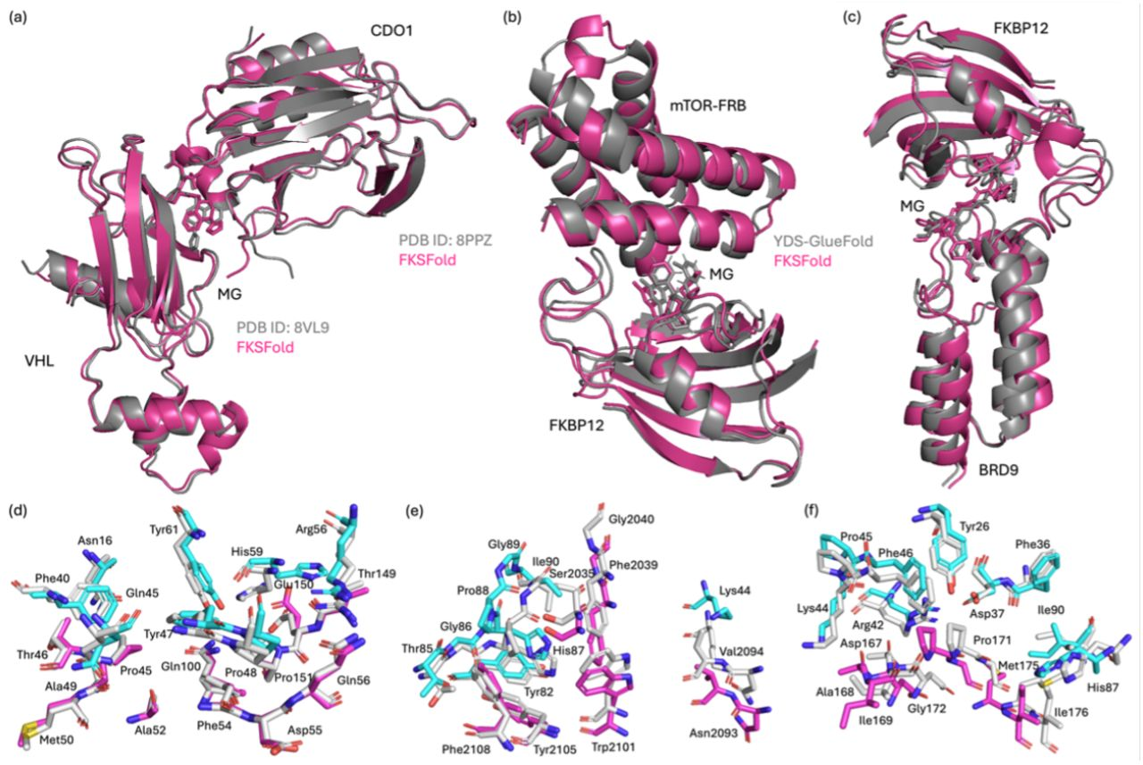
蛋白的序列文件,FASTA格式,支持多条序列。
注意:多蛋白复合物结构预测,其氨基酸序列输入格式如下:
>protein1
AASJ...
>protein2
AASJ...
>peptide
ASDF...
DNA核酸的序列文件,FASTA格式,支持多条序列。
RNA核酸分子的序列文件,FASTA格式,支持多条序列。
备注:当前24GB的GPU显存能计算的残基/碱基数量在2048个左右。
在Protein、DNA、RNA序列中,都支持残基或碱基的修饰,用CCD进行定义,CCD的介绍参考https://www.wwpdb.org/data/ccd 编号查询网址为https://www.ebi.ac.uk/pdbe-srv/pdbechem/
定义残基或碱基修饰时,直接在序列中用英文括号‘()’包含CCD code即可,示例如下:
>seq
(ACE)GQLEEIAK
表示在序列的N端发生了乙酰化;
>seq
AGSHSMRYFSTSVSR(HY3)GRGEPRFIAVG
表示序列中的残基P发生了羟基化修饰,变成HY3(CCD code)
文本文件包含小分子的结构信息,用SMILES格式,支持多个小分子,每行放置一个,示例如下:
CC(=O)OC1C[NH+]2CCC1CC2
[Mg+2]
注意:不适用于配体蛋白或多肽的氨基酸序列格式输入。
包含残基间距离限制信息的文本文件。距离限制的类型有两种:两个残基间的距离限制,一个残基与一条链之间的距离限制。
两个残基间的距离限制的定义由五部分组成:
五部分由逗号分隔,例如:1,R84,3,G7,10.0
表示第1条序列中的84号残基R,与第3条序列中的7号残基G,之间的最大距离为10.0埃。
一个残基与一条链之间的距离限制表示该残基与链中任意一个残基的距离满足限制即可。其定义方式与上述类似,差异在于,残基1与残基2的符号及位置编号,其中一个需设置为0(不可同时为0),例如:1,R84,3,0,10.0
表示第1条序列中的84号残基R,与第3条链的任意一个残基/碱基的最大距离为10.0埃即可。
支持放置多个距离限制,每行放置一个即可,包含多个距离限制信息的文件内容示例如下:
1,H189,3,L4,8.0
1,R84,3,0,10.0
输出结果文件为排名前5的复合物结构rank_1-5.cif和pred_scores_chai1.csv,csv中包含信息如下:
| 列名 | 说明 |
|---|---|
| Name | 结构名称 |
| aggregate_score | 对预测结构的质量排序的指标分数,值范围在-100至1.0之间,越大表示预测结构的质量越高。该分数综合考虑了三个指标:ptm, iptm, has_clash, 计算公式为: Aggregate_Score = 0.8 × ipTM + 0.2 × pTM − 100 × has_clash |
| ptm | 预测的TM分数(the predicted template modeling score),衡量预测结构整体准确性,越大表示越准确,该分数大于0.5时,表示结构整体折叠可能与真实结构相似 |
| iptm | 预测的亚基接触面的TM分数(the interface predicted template modeling score),当预测结构为复合物时才有该评价指标,衡量复合物中各个亚基之间相对位置的预测准确性,越大表示越准确,大于0.8表示高质量预测,小于0.6表示预测可能失败,0.6-0.8为灰色地带,预测正确与否不确定 |
| per_chain_ptm | 每条链单独计算的 pTM 分数,用于评估复合物中各个单链结构折叠预测的可靠性。该值可用于判断某一条链是否预测质量较低。 |
| per_chain_pair_iptm | 每一对链之间的 界面 ipTM 分数矩阵,用于评估复合物中不同链对之间相互作用界面的预测可靠性。 |
| has_inter_chain_clashes | 是否存在 跨链原子碰撞(inter-chain clashes) 的标志。通常为布尔值或 0/1。若存在碰撞(1),说明不同链之间存在严重空间重叠,结构可能不合理。 |
| chain_chain_clashes | 各链之间发生的 原子碰撞数量或碰撞统计信息,用于进一步评估复合物界面是否存在结构冲突。 |
| actif_ptm | 用于衡量复合物预测中 参与相互作用界面的区域结构质量。相比整体 pTM,更关注界面区域结构的可靠性。 |
| mean_interface_ptm | 所有预测界面区域的 平均 pTM 分数,用于整体评估复合物界面结构的可靠性。 |
| protein_mean_interface_ptm | 仅针对 蛋白质链之间界面 计算的平均 interface pTM 分数,用于评估蛋白–蛋白相互作用界面预测质量。 |
| pae_scores | 用于表示模型预测中不同残基之间的相对位置误差。数值越低表示预测越可靠,常用于分析结构域之间或链之间的相对定位可信度。 |
A structure prediction model developed based on Chai-1, specifically designed for molecular glue complex systems. By integrating Feynman-Kac (FK) stochastic control theory with AlphaFold3’s diffusion model, it introduces the interface prediction TM-score (ipTM) to evaluate the quality of protein-protein interfaces in real-time during the generation process. It modifies the reverse diffusion process using guidance terms derived from the FK formula to prioritize the preservation of high-scoring structures. Meanwhile, the FK framework enables the sampling to be biased toward biophysically plausible conformations without requiring extensive retraining of the underlying model or compromising the diversity of generated structures. This method successfully predicted three out of eight molecular glue cases with an RMSD of less than 3Å.
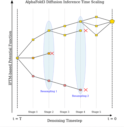
The sequence file of proteins in FASTA format, supporting multiple sequences.
Note: For multi-protein complex structure prediction, the amino acid sequence input format is as follows:
>protein1
AASJ...
>protein2
AASJ...
>peptide
ASDF...
The sequence file of DNA nucleic acids in FASTA format, supporting multiple sequences.
The sequence file of RNA nucleic acid molecules in FASTA format, supporting multiple sequences.
** Note: Current 24GB GPU memory can calculate around 2048 residues/bases. **
In Protein, DNA, RNA sequences, all support the modification of residues or bases, which are defined by CCD, The introduction of the CCD reference https://www.wwpdb.org/data/ccd Number query url for https://www.ebi.ac.uk/pdbe-srv/pdbechem/
To define a residue or base modification, simply include the CCD code in parentheses’ () 'in the sequence, as shown in the following example:
>seq
(ACE)GQLEEIAK
Indicates acetylation at the N-terminus of the sequence;
>seq
AGSHSMRYFSTSVSR(HY3)GRGEPRFIAVG
Indicates that residue P in the sequence is hydroxylated and becomes HY3 (CCD code).
The text file contains structural information about small molecules, in SMILES format, supporting multiple small molecules, one per line, as shown in the following example:
CC(=O)OC1C[NH+]2CCC1CC2
[Mg+2]
Note: Not applicable for amino acid sequence format input of ligand proteins or polypeptides.
The five parts are separated by commas, for example: 1,R84,3,G7,10.0
Denote residue 84 R in the first sequence, and residue 7 G in the third sequence, with a maximum distance of 10.0 angstroms.
** The distance limit between a residue and a chain ** means that the distance between the residue and any residue in the chain satisfies the limit. It is defined in the same way as above, except that the symbol and position number of residue 1 and residue 2 need to be set to 0 (not both), e.g. 1,R84,3,0,10.0
Denotes residue 84 R in the first sequence, and a maximum distance of 10.0 angstroms from any residue/base of the third strand is sufficient.
Multiple distance limits are supported, one per line, and an example file containing multiple distance limits is as follows:
1,H189,3,L4,8.0
1,R84,3,0,10.0
| Field Name | Description |
|---|---|
| Name | Name of the complex structure |
| Aggregate_Score | Index scores that rank the quality of the predicted structure, with values ranging from -100 to 1.0, with larger values indicating higher quality of the predicted structure. The score takes into account three metrics: ptm, iptm, has_clash, and is calculated as follows: Aggregate_Score = 0.8 × ipTM + 0.2 × pTM − 100 × has_clash |
| pTM | The predicted template modeling score, which measures the overall accuracy of the predicted structure. A higher score indicates greater accuracy. If the score is greater than 0.5, it suggests that the overall folding of the structure may be similar to the true structure. |
| ipTM | The interface predicted template modeling score, which measures the accuracy of the predicted relative positions of the subunits in the complex. A higher score indicates greater accuracy. Scores above 0.8 indicate high-quality predictions, while scores below 0.6 suggest potential failure of the prediction. Scores between 0.6 and 0.8 are in a gray area, where the accuracy of the prediction is uncertain. |
| per_chain_ptm | The pTM score calculated for each individual chain, used to assess the structural reliability of each monomer within the complex. |
| per_chain_pair_iptm | A matrix containing ipTM scores for each pair of chains, used to evaluate the reliability of predicted interfaces between specific chain pairs. |
| has_inter_chain_clashes | A boolean or binary indicator (0/1) showing whether steric clashes occur between atoms of different chains. If clashes are present, the predicted complex structure may be physically unrealistic. |
| chain_chain_clashes | The number or statistics of atomic clashes between chains, providing more detailed information about structural conflicts at the interfaces. |
| actif_ptm | Active interface pTM, representing the predicted structural confidence specifically for residues involved in interaction interfaces. |
| mean_interface_ptm | The average pTM score across all predicted interaction interfaces, providing an overall estimate of interface structural reliability. |
| protein_mean_interface_ptm | The average interface pTM specifically for protein–protein interfaces, used to assess the quality of predicted protein interaction regions. |
| pae_scores | Predicted Aligned Error (PAE) matrix, representing the expected positional error between residue pairs. Lower values indicate higher confidence in the relative positioning of residues or domains. |
基于BsAb双抗序列编辑器输出的序列格式,进行双抗结构预测,当前支持含IgG的对称性双抗结构预测。
Based on the sequence format output by the BsAb bispecific antibody sequence editor, this module performs bispecific antibody structure prediction. Currently, it supports structure prediction for symmetrical bispecific antibodies containing IgG.

预测抗体-抗原复合物结构的DockQ值,进行结构质量评价。模块基于DeepRank-Ab模型实现,DeepRank-Ab是一种专为抗体 - 抗原界面独特特性量身定制的几何深度学习评分函数。该函数的开发得益于一个精心构建的基准数据集,该数据集包含来自 1442 个复合物的 230 多万个诱饵构象,为稳健训练和无偏评估提供了所需的多样性。在多个独立测试集(包括非结合态 - 非结合态对接模型和 AlphaFold 生成的结构)上,DeepRank-Ab 持续优于所有评估方法,包括 AF3、HADDOCK 以及 FTDMP 等最先进的评分函数。它将 AF3 的 Top 1 成功率提升了 35.5%,并将平均 Top 1 DockQ 值提高了一倍以上。DeepRank-Ab 还能稳健泛化到训练分布之外,在外部抗体 - 抗原 CAPRI 靶点上实现 100% 的 Top 5 成功率,超越了所有测试方法。这些结果共同表明,DeepRank-Ab 是一种高效的评分方法,显著提升了近天然抗体 - 抗原构象的识别能力。

抗体/纳米抗体-抗原复合物结构文件,支持格式:.pdb、.cif、.pdb.gz、.cif.gz,支持批量结构,要求以压缩包形式输入,支持格式:.zip、.tar、.tar.gz、.tgz、.tar.bz2、.tbz2、.tar.xz、.txz
输出deeprank_ab_result.csv,内容如下:
| Name | Predicted DockQ |
|---|---|
| test1 | 0.20 |
| test2 | 0.17 |
| 字段 | 说明 |
|---|---|
| Name | 结构/样本标识符,PDB 名称。 |
| Predicted DockQ | DeepRank-Ab 预测的 DockQ 分数(数值越高通常表示复合物对接质量越好;范围常见在 0–1)。 |
Predicts the DockQ score of antibody–antigen complex structures for structural quality assessment. This module is based on the DeepRank-Ab model, a geometric deep learning scoring function specifically designed for the unique characteristics of antibody–antigen interfaces. The development of this function is supported by a carefully curated benchmark dataset containing over 2.3 million decoy conformations from 1,442 complexes, providing the necessary diversity for robust training and unbiased evaluation.
On multiple independent test sets, including unbound–unbound docking models and AlphaFold-generated structures, DeepRank-Ab consistently outperforms all evaluation methods, including state-of-the-art scoring functions such as AF3, HADDOCK, and FTDMP. It improves AF3’s Top 1 success rate by 35.5% and more than doubles the average Top 1 DockQ score. DeepRank-Ab also generalizes robustly beyond the training distribution, achieving a 100% Top 5 success rate on external antibody–antigen CAPRI targets, outperforming all tested methods. These results collectively demonstrate that DeepRank-Ab is an efficient scoring approach that significantly enhances the recognition of near-native antibody–antigen conformations.
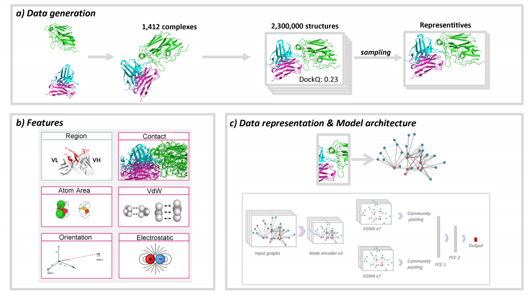
Antibody–antigen and nanobody–antigen complex structure files are supported in the following formats: .pdb, .cif, .pdb.gz, .cif.gz.
Batch submission of multiple structures is supported and must be provided as a compressed archive. Supported archive formats include: .zip, .tar, .tar.gz, .tgz, .tar.bz2, .tbz2, .tar.xz, .txz.
Generates deeprank_ab_result.csv with the following content:
| Name | Predicted DockQ |
|---|---|
| test1 | 0.20 |
| test2 | 0.17 |
| Field | Description |
|---|---|
| Name | Structure/sample identifier, typically the PDB name. |
| Predicted DockQ | DockQ score predicted by DeepRank-Ab (higher values generally indicate better docking quality; typical range 0–1). |
Grafting模块是移植抗体的CDR到特定的框架区模板上,通常用于人源化设计。版本:v2.5
抗体序列文件,FASTA格式
抗体编号规则:kabat,imgt,chothia
指定输出抗体graft后的序列文件名称,FASTA格式
指定输出graft策略文件,JSON格式
指定输出抗体FR区序列比对同源性打分文件
指定轻链或重链使用特定germline模板,也可都指定,写法如下:
seq_name1:germline_name1,seq_name2:germline_name2
其中链名来自于流程第一步输入的fasta文件。
例1:以下语句为链"Infliximab.H"指定了模板"IGHV3-7*01":
Infliximab.H:IGHV3-7*01
例2:以下语句为两条链分别指定了模板:
Infliximab.H:IGHV3-7*01,Infliximab.L:IGKV1-39*01
指定抗体可变区 V 基因 的参考模板序列,FASTA格式。
指定抗体可变区 J 基因 的参考模板序列,FASTA格式。
指定输出FR区序列比对结果文件,FASTA格式
指定输出命中序列的数目
输出结果包括:
| 输出文件名称 | 说明 |
|---|---|
| germline_hits.fasta | 输出FR区序列比对结果文件 |
| germline_score.json | 输出抗体FR区序列比对同源性打分文件 |
| grafted.fasta | 输出抗体graft后的序列文件名称 |
| graft_policy.json | 输出graft策略文件 |
| Germline Frequency | germline 模板打分未知残基频率 |
The Grafting module is used to graft the CDRs of an antibody onto a specific framework region template, typically used for humanization design. Version: v2.5
Antibody sequence file in FASTA format.
Antibody numbering rule: kabat, imgt, chothia.
Specify the output file name for the grafted antibody sequence in FASTA format.
Specify the output grafting strategy file in JSON format.
Specify the output file for the homology scores of the antibody FR region sequences.
Specify the specific germline template to be used for the light chain or heavy chain, or both, in the format:
seq_name1:germline_name1,seq_name2:germline_name2
Where the chain names come from the FASTA file input in the first step of the process.
Example 1: The following statement specifies the template “IGHV3-7*01” for the chain “Infliximab.H”:
Infliximab.H:IGHV3-7*01
Example 2: The following statement specifies templates for two chains separately:
Infliximab.H:IGHV3-7*01,Infliximab.L:IGKV1-39*01
Specify the reference template sequence of the antibody V gene in FASTA format.
Specify the reference template sequence of the antibody J gene in FASTA format.
Specify the output file for the FR region sequence alignment results in FASTA format.
Specify the number of sequences to output.
The output includes:
| Output File Name | Description |
|---|---|
| germline_hits.fasta | Output file for FR region sequence alignment results |
| germline_score.json | Output file for homology scores of the antibody FR region sequences |
| grafted.fasta | Output file name for the grafted antibody sequence |
| graft_policy.json | Output file for the grafting strategy |
| Germline Frequency | Frequency of unknown residues in germline template scoring |
设计能够结合各种生物分子靶标的蛋白、肽类等生物分子。模块基于BoltzGen模型实现,BoltzGen是一个通用的全原子生成模型(all-atom generative model),能够在同一框架下完成多模态的binder设计任务。不同于前代模型只做“推断”,BoltzGen直接在扩散采样过程中生成目标分子与其结合体的全原子结构,并通过可控约束机制确保生成结果物理一致、功能可实现。同时具备良好的泛化性能,能够针对训练过程中未出现过的全新靶标进行有效设计。
BoltzGen的方法设计承接了Boltz系列一贯的目标——在统一的几何表示与能量空间中,学习多模态分子的物理规律。与以往的预测模型不同,BoltzGen 并不输出单一结构预测,而是通过扩散建模(diffusion modeling)直接生成分子的全原子坐标。
其采用扩散模型(diffusion model)框架,在全原子坐标空间中学习分子结构的分布。模型通过在每个采样步骤中向原子坐标加入高斯噪声,再逐步去噪恢复,从而近似真实的势能面分布。与传统的分子生成模型(如仅在残基层面建模)不同,BoltzGen的每个采样变量都是具体原子的位置向量。模型通过能量一致性约束(energy consistency)学习键长、键角、二面角等局部几何关系,从而在生成时自动保持化学合理性。这里对于全原子建模采用了Atom14的方法。
这一设计使生成结构不仅在形状上接近真实蛋白,在能量上也符合分子物理规律。
BoltzGen的架构如下图所示,由三大模块组成:输入层(Input Representation)、条件编码器(Condition Encoder)、扩散模型(Diffusion Model),输出为三维坐标的全原子结构。
BoltzGen的一个突出特点,是并非停留在计算层面的生成验证,而是进行了系统的湿实验评估。进行了十类实验任务(如下图所示),涵盖 蛋白质、肽类、环肽、小分子结合体及抗菌肽设计等多种体系,几乎囊括了现有结构设计模型所能覆盖的全部生物模态。这些实验的共同目标,是检验模型能否在“无同源模板、真实实验条件”下生成可表达、可结合的结构。不同于以往只验证折叠精度的预测模型,BoltzGen的验证标准是功能实现——即所生成分子是否能在实验中稳定结合目标。
BoltzGen 的实验结果显示出较高的一致性与通用性:
在 BoltzGen 论文中,进行抗体和结合蛋白生成的湿实验验证时,抗原(目标蛋白)的主要输入方式是结构,但在特定情况下也可以通过序列输入。
具体说明如下:
默认输入方式:结构
论文中明确提到,除非另有说明,实验中均是将目标的结构(structure)作为输入提供给 BoltzGen 。例如,在针对 9 个新型目标(Novel Targets)设计纳米抗体和蛋白质结合剂时,研究人员利用了目标的结构信息。
灵活性:序列输入与协同折叠(Cofolding) BoltzGen 是一个全原子生成模型,能够同时进行结构预测和蛋白质设计 。当仅提供目标的序列(sequence)作为输入时,模型可以在设计结合剂的同时对目标进行折叠,最终生成结合复合物的原子结构 。
特殊案例:
总结来说,虽然BoltzGen具备直接从序列出发进行设计的能力,但在该论文的大多数湿实验验证(特别是针对新型蛋白目标)中,结构是主要的输入方式。
| 抗原大小 | 生成模式 | 生成序列数量 | 计算耗时(小时) |
|---|---|---|---|
| 120 | Nanobody | 10000 | 4.5 |
| 140 | Nanobody | 10000 | 5.0 |
| 180 | Nanobody | 10000 | 6.0 |
| 200 | Nanobody | 10000 | 6.5 |
| 400 | Nanobody | 10000 | 11.5 |
| 460 | Nanobody | 10000 | 15.0 |
| 240 | Antibody | 10000 | 10.8 |
| 290 | Antibody | 10000 | 15.0 |
| 400 | Antibody | 10000 | 17.5 |
指定抗体类型,目前支持Antibody(普通抗体)和Nanobody(纳米抗体)。
上传已有的抗原结构,PDB或CIF格式。
指定从结构中提取一些链作为抗原,可多选,如:A,B。如不设置该参数,表示提取结构中的所有链。
如果没有已知的抗原结构,可上传抗原序列,fasta格式,支持多链。
指定抗原中的哪些残基参与结合,使用链名+残基位置(从1开始的顺序编号)进行指定,如A10-20,A25,B30-36,B40。
表示:抗原结合位点为A链编号10至20、25的残基,B链提编号30至36、40的残基。
注意:
1,在使用抗原序列文件时,链名是按字母顺序命名(与链的位置顺序对应),第一条链的链名为A,第二条链的链名为B,依次命名。
2,如不设置该参数,模型会自主寻找潜在的结合位点。
支持上传自定义的抗体或纳米抗体模板结构,会采用模板结构的FR区,对CDR区域(Chothia编号)进行重设计,可选择:
.pdb 或 .cif)多个模板结构时,每个模板结构都会用于设计。Number of Samples参数若设为10000,在默认抗体模板的情况下,每个模板结构的次数都约为3333。
如未提供自定义模板,系统将使用内置的默认抗体模板和纳米抗体模板,具体如下:
抗体模板:
6CR1 — Adalimumab(阿达木单抗,Humira)
靶点:TNF-α
作用:阻断 TNF-α 与受体结合,抑制炎症反应
6WGB — Dupilumab(度普利尤单抗,Dupixent)
靶点:IL-4Rα
作用:阻断 IL-4 / IL-13 信号通路,抑制 2 型炎症
3HMW — Ustekinumab(乌司奴单抗,Stelara)
靶点:IL-12 / IL-23 p40
作用:同时抑制 Th1 和 Th17 炎症通路
纳米抗体模板:
7EOW — Caplacizumab(卡普赛珠单抗)
靶点:vWF A1 域
作用:阻断 vWF 与血小板结合,抑制血栓形成
7XL0 — Vobarilizumab(ALX-0061,沃巴利珠单抗)
靶点:IL-6R(+ 白蛋白结合)
作用:抑制 IL-6 信号并延长半衰期
8COH — TPP-3444(Gefurulimab / ALXN1720 组成部分)
靶点:补体 C5
作用:抑制补体激活
8Z8V — ALB8(Ozoralizumab / ATN-103 组件)
靶点:人血清白蛋白(HSA)
作用:延长药物半衰期
Gontivimab(ALX-0171,格替韦单抗)
靶点:RSV F 蛋白
作用:阻断病毒融合,抑制感染
Isecarosmab(M-6495 / ALX-1141,艾司卡索单抗)
靶点:ADAMTS-5
作用:抑制软骨降解,具有抗炎作用
Sonelokimab
靶点:IL-17A / IL-17F
作用:双重抑制炎症因子,增强抗炎效果
采样的序列数量,值越大,采样空间越大,筛选序列质量越高,对应计算时间也更长,最大支持20000。
完成设计后,最终给出的结构数量,默认为30,最大支持100。
设计模式共有6种:
设计规则的定义有三种方式:
三种方式可以自由组合。
上传已有蛋白结构,从中提取已有结构,或重新设计部分结构。例如:从上传的结构中提取靶点链、抗原链、纳米抗体链等。
指定从Structure中提取的链名,可多选,如:A,B。如不设置该参数,表示提取结构中的所有链。
从Chains参数指定的链中,进一步确认需要提取的残基范围,使用链名+残基位置(从1开始的顺序编号,非PDB的UID编号)进行指定,如A10-20,A25,B1-36,B40。
表示:从A链提取编号10至20、25的残基,从B链提取编号1至36、40的残基。
如不设置该参数,表示提取Chains参数中指定的完整链。
从Chains参数指定的链中,确认哪些残基不提取),与Include参数作用相反,指定方式相同,如A15,B36-42(从1开始的顺序编号,非PDB的UID编号表示A链编号15、B链编号36至42的残基不提取。
已提取的结构中,指定需要重新设计的残基,指定方式同Include参数,如A10-12,B15,B40(从1开始的顺序编号,非PDB的UID编号)。
注意:需要重新设计的残基编号应在已提取的结构中存在。
对要设计的残基,指定二级结构类型。使用链名,SS类型:残基范围(从1开始的顺序编号,非PDB的UID编号)进行指定,每行放置一个,如:
A,HELIX:10-12
B,SHEET:15,LOOP:40
二级结构类型可选:LOOP, HELIX, SHEET(大小写均可)。
不指定该参数表示不强制二级结构类型。
指定哪些残基参与结合(如链间或与小分子结合),指定方式同Include,如A12,B15-18(从1开始的顺序编号,非PDB的UID编号)。
指定哪些残基不参与结合(从1开始的顺序编号,非PDB的UID编号),与Binding参数作用相反。
指定插入突变设计,使用链名,插入位置,插入残基长度,二级结构(从1开始的顺序编号,非PDB的UID编号方式定义,每行一个,如:
A,10,5
B,15,5-10,HELIX
表示在A链的10号残基位置后,插入5个新残基,二级结构不确定(不强制)。在B链的15号残基位置后,插入5至10个残基(具体残基数量随机确定),二级结构为HELIX。
二级结构类型的选择有3种(大小写皆可): LOOP, HELIX, or SHEET
同Structure定义。例如:指定已有的Binder结构。
同Chains定义
同Include定义
同Exclude定义
同Design Positions定义
同Design SS定义
同Binding Hotspot定义
同Non Binding定义
同Design Insertions定义
指定要设计的蛋白序列,每行一条,如:
AAVTTTTPPP
15-20AAAAAAVTTTT18PPP
其中:
18表示序列的该位置将设计18个残基。15-20表示该位置将设计15至20个残基,具体长度在15至20之间随机指定。序列的ID默认从1开始按顺序编号。
指定序列中参与结合的残基,使用序列编号:残基范围格式,如:
1:5,8-10
2:30-35
表示第一条序列中编号5、8至10的残基参与结合;第二条序列中编号30至35的残基参与结合。
第二条序列中含有设计长度范围时,按最小长度计算残基位置。
指定序列中不参与结合的残基,与Sequence_Binding作用相反。
指定序列中残基的二级结构类型,使用序列编号,SS类型:残基范围定义,每行一条,如:
1,HELIX:5-8
2,SHEET:15,LOOP:40
表示第一条序列编号5至8的残基,二级结构为HELIX;第二条序列编号15的残基,二级结构为SHEET,编号40的残基,二级结构为LOOP。
注意: 有指定设计长度范围的序列,按长度最小值来确认剩余残基的位置。
指定需要环化的序列编号,如1,2表示第1和第2条序列首尾相连。
指定参与结合的小分子信息,文本文件,支持SMILES或 CCD Code(化学组分词典编号)。如果使用SMILES格式,每行应包含一个小分子;如果使用CCD Code,每行可以包含一个或多个小分子,使用逗号分隔,并加上CCD前缀。示例如下:
CC(=O)OC1C[NH+]2CCC1CC2
CCD,ATP,HY3,P1L
CCD,MG
共价键信息的文本文件,TXT格式。每行放置一个共价键信息,每个共价键信息包含两个原子信息,每个原子信息由三部分组成:
3,1,CA表示第三个实体(序列或小分子)中的第一个残基(或小分子)的CA原子1,1,CA;2,1,CA1,1,CA,第二个原子为2,1,CA1,1,CA;2,1,CA
1,1,CA;3,1,CHA
当小分子为SMILES时,如CC(=O)NCCNC(C)=O,如果该小分子的顺序编号(按上述方式确认)为3,其第一个C原子参与形成共价键,与编号为1的链/序列中第一个残基的CA原子,则共价键的定义为1,1,CA;3,1,C1其中C1表示小分子的第一个C原子,如果是第二C原子,用C2表示。
注意:
15-20ACS,长度范围的序列长度按最小长度计算,即15,所以残基A的位置编号是16,C是17,S是18。采样的序列数量,值越大,采样空间越大,筛选序列质量越高,对应计算时间也更长,最大支持20000。
完成设计后,最终给出的结构数量,默认为30,最大支持100。
输出参数文件design_spec.yaml
输出设计的复合物的序列文件,final_complex.fasta
输出设计的复合物的序列文件(Batch模式),final_complex_batch.fasta,适合一些模块的Batch模式的输入,如Structure Prediction (Boltz-2)
输出设计的链的序列文件,final_designed_chains.fasta
输出设计打分文件final_designs_metrics.csv,csv文件每个指标含义如下:
| 列名 | 说明 |
|---|---|
| id | 设计分子的名称 |
| final_rank | 通过各指标综合排序后的最终排名 |
| absolute_score | 基于多种指标(结构指标,物理能量指标)计算的综合打分,但与final rank排序并不完全一致,供参考。 |
| structure_confidence | 基于结构指标(ptm,iptm,pae)计算的结构置信度评分,供参考。 |
| design_ptm | 设计结构的预测TM分数(0–1),反映模型对设计蛋白整体折叠结构的置信度。数值越高表示设计结构越合理,通常 >0.7 视为高置信度。 |
| design_iptm | 设计结构与靶点结构相互作用界面的预测TM分数(0-1),反应相互作用界面质量的置性度。数值越高表示界面结构越合理,通常 >0.7 视为高置信度。 |
| design_to_target_iptm | 仅设计的残基与靶点结构相互作用界面的预测TM分数(0–1),反应相互作用界面质量的置性度。数值越高表示界面结构越合理,通常 >0.7 视为高置信度。 |
| min_design_to_target_pae | 最小预测对齐误差(Å),是残基对水平的置信度指标,用来衡量任意两个残基之间相对空间位置的预测可信度。这里表示设计的结构与靶点结构的残基之间相对位置的准确度。数值越小(例如 <10 Å)准确度越高。 |
| plip_saltbridge_refolded | 重折叠后结构中的盐桥数量。盐桥(带相反电荷残基间的电性作用力)是维持蛋白稳定性的重要因素,数量越多通常结合越稳固。 |
| plip_hbonds_refolded | 重折叠后结构中的氢键数量。氢键是二级结构和界面互补性的关键作用力,数量越多整体稳定性越好。 |
| delta_sasa_refolded | 重折叠前后溶剂可及表面积变化(ΔSASA, Ų)。数值越大(例如 >2000 Ų)表示疏水核心包埋程度越高,通常代表更强的热稳定性。 |
| filter_rmsd | 整个复合物(设计+靶点)结构重折叠后与原设计结构的RMSD值,用于验证生成结构与预测结构的一致性,数值越小越好。 |
| design_ipsae_min | 设计结构与靶点结构之间的最小ipSAE数值(从设计结构出发,计算与靶点结构之间的ipSAE,反之从靶点结构出发,计算与目标结构之间的ipSAE,两者中取最小值)。ipSAE是基于pAE(predicted Aligned Errors)矩阵计算得到的相互作用界面评价分数,取值范围是0到1,值越大,表示预测的蛋白-蛋白相互作用界面越可靠。ipSAE > 0.7 表明相互作用界面预测质量高,结构可信。ipSAE < 0.1: 表明预测中几乎不存在可信互作界面,可排除假阳性相互作用。 |
| design_to_target_ipsae | 从设计结构出发,计算与靶点结构之间的ipSAE。 |
| ALA/GLY/GLU/LEU/VAL/CYS_fraction | 设计的残基中,各类型氨基酸的比例 |
| contacts | 预测结构中的接触界面残基 |
| contacts_overlap | 与输入 hotspot 重叠的预测接触残基 |
| overlap_ratio | 输入 hotspot 被预测接触残基覆盖的比例 |
注意:只有设置Binding Hotspot参数,才会输出
输出设计的前5个结构rank1-5*.cif
输出最后设计的结构打包文件final_designs.tar.gz
输出设计的概述文件results_overview.pdf,包含结构的过滤 (Filtering Criteria)和排序标准(Sorting Criteria)。
| 列名 | 说明 |
|---|---|
| has_x | 阈值:0.0 序列有效性检查。确保序列中不包含未知氨基酸(“X”),必须完全由标准的 20 种天然氨基酸组成,保证序列在物理上可被合成和表达。 |
| filter_rmsd | 阈值:< 2.5 Å 整体骨架的 RMSD。检查整个复合物(设计+靶点)在重折叠后是否保持原样,用于验证生成结构与预测结构的一致性。 |
| filter_rmsd_design | 阈值:< 2.5 Å 仅针对设计部分(Binder)的骨架 RMSD。确保即使靶点有微小移动,结合剂本身的结构依然是稳定的。 |
| designfolding-filter_rmsd | 阈值:< 2.5 Å 独立折叠稳定性检查。在没有靶点的情况下单独折叠结合剂并计算 RMSD。用于确保结合剂能独立折叠,从而大大提高湿实验中的表达成功率。 |
| ALA_fraction GLY_fraction GLU_fraction LEU_fraction VAL_fraction |
阈值:< 0.3 (30%) 序列复杂度/多样性检查。限制丙氨酸、甘氨酸、谷氨酸、亮氨酸、缬氨酸的单项占比。防止模型为了刷高结构稳定性分数而生成单一重复序列,强制要求序列具备化学多样性,以保证特异性的相互作用能力。 |
| 列名 | 说明 |
|---|---|
| design_to_target_iptm | 权重为1 界面预测 TM 得分(0–1),用于评估蛋白–蛋白相互作用界面的结构合理性。数值越大表明界面(如结合位点)越可能形成稳定相互作用。 |
| design_ptm | 权重为1 预测模板建模得分(0–1),反映模型对设计蛋白整体折叠结构的置信度。数值越高表示全局结构越合理,通常 >0.7 视为高置信度。 |
| neg_min_design_to_target_pae | 权重为1 负的最小界面预测对齐误差 (PAE)。PAE 越低越好(误差越小),取负值是为了方便排序(数值越大越好)。它代表模型对结合界面上“最确定的那个接触点”有多大把握。 |
| affinity_probability_binary1 | 权重为1 亲和力预测概率。主要用于小分子结合剂场景。这是模型直接预测出的“该分子能结合”的概率值。 |
| plip_hbonds_refolded | 权重为0.5 重折叠后结构中的氢键数量。氢键是二级结构和界面互补性的关键作用力,数量越多整体稳定性越好。 |
| plip_saltbridge_refolded | 权重为0.5 重折叠后结构中的盐桥数量。盐桥(带相反电荷残基间的电性作用力)是维持蛋白稳定性的重要因素,数量越多通常结合越稳固。 |
| delta_sasa_refolded | 权重为0.5 重折叠前后溶剂可及表面积变化(ΔSASA, Ų)。数值越大(例如 >2000 Ų)表示疏水核心包埋程度越高,通常代表更强的热稳定性。 |
1. 抗体编号
应用WeView打开mH35抗体结构,进行抗体编号,确定重链CDR3的位置在H99-102,为遮蔽肽的结合位置
2. BoltzGen中输入参数设置
1. 抗体编号
应用WeSeq打开mH35抗体序列,进行抗体编号,确定重链CDR3的位置在99-102,为遮蔽肽的结合位置
2. BoltzGen中输入参数设置
The Binder Design module is designed to generate proteins, peptides, and other biomolecules capable of binding to various biological targets. It is implemented based on the BoltzGen model — a universal all-atom generative model capable of performing multimodal binder design tasks within a unified framework. Unlike earlier models that focused solely on “inference,” BoltzGen directly generates the full-atom structures of target molecules and their complexes during diffusion sampling, ensuring physically consistent and functionally feasible results through controllable constraints. It also demonstrates strong generalization, enabling effective design for novel, unseen targets.
The BoltzGen framework inherits the Boltz family’s core objective — to learn the physical laws of multimodal molecules within a unified geometric and energetic representation. Unlike traditional prediction models that output a single structure, BoltzGen uses diffusion modeling to directly generate full atomic coordinates of molecules.
BoltzGen adopts a diffusion model framework to learn molecular structure distributions in full-atom coordinate space. The model adds Gaussian noise to atomic coordinates at each sampling step and progressively denoises them to approximate the real potential energy surface. Unlike traditional residue-level molecular generators, BoltzGen models each atom’s position explicitly. Using energy consistency constraints, the model learns local geometric relationships — such as bond lengths, angles, and torsions — to ensure chemical plausibility during generation. The Atom14 method is used for full-atom representation.
This design ensures that generated structures are not only geometrically realistic but also physically valid in terms of molecular energetics.
The BoltzGen architecture consists of three main modules: Input Representation, Condition Encoder, and Diffusion Model, outputting full-atom 3D coordinates.
A distinguishing feature of BoltzGen is that it goes beyond computational validation and includes extensive wet-lab experimental evaluation. Ten categories of experiments were performed (as shown below), covering proteins, peptides, cyclic peptides, protein–small molecule complexes, and antimicrobial peptides — encompassing nearly all biological modalities addressed by structural design models. The goal was to test whether BoltzGen can generate expressible, functional binders under real experimental conditions without any homologous templates. Unlike models that only validate structural accuracy, BoltzGen emphasizes functional success — i.e., whether the generated molecules can stably bind their targets experimentally.
Experimental results demonstrate high consistency and generality:
In the BoltzGen paper, during wet-lab validation of antibody and binder generation, the primary form of input for the antigen (target protein) is structural information, although sequence-only input is also supported in specific scenarios.
Default Input Mode: Structure
The paper explicitly states that, unless otherwise specified, the target structure is provided as input to BoltzGen in the experiments. For example, when designing nanobodies and protein binders against nine novel targets, the researchers relied on the structural information of the targets.
Flexibility: Sequence Input and Cofolding
BoltzGen is an all-atom generative model capable of performing structure prediction and protein design simultaneously. When only the target sequence is provided, the model can cofold the target and the binder, folding the target while designing the binder and ultimately generating the atomic structure of the bound complex.
Special Cases
No Fixed Structure Input
When designing peptides targeting the disordered region of the NPM1 protein, the researchers adopted a “no fixed structure input” strategy. They provided the structure of the ordered regions of NPM1 while leaving the disordered region flexible, allowing the model to evaluate performance on targets lacking a well-defined structure.
Small-Molecule Targets
For small-molecule targets, BoltzGen requires only a SMILES string (a sequence-based representation of molecular structure) as input and performs cofolding during the design process.
In summary, although BoltzGen is capable of performing design directly from sequence-only inputs, in the majority of the wet-lab validation experiments reported in the paper—especially those involving novel protein targets—structural information was used as the primary form of input.
| Antigen Size | Generation Mode | Number of Sequences | Computation Time (hours) |
|---|---|---|---|
| 120 | Nanobody | 10000 | 4.5 |
| 140 | Nanobody | 10000 | 5.0 |
| 180 | Nanobody | 10000 | 6.0 |
| 200 | Nanobody | 10000 | 6.5 |
| 400 | Nanobody | 10000 | 11.5 |
| 460 | Nanobody | 10000 | 15.0 |
| 240 | Antibody | 10000 | 10.8 |
| 290 | Antibody | 10000 | 15.0 |
| 400 | Antibody | 10000 | 17.5 |
Specifies the antibody type. Currently supports Antibody (conventional antibodies) and Nanobody.
Upload an existing antigen structure in PDB or CIF format.
Specify which chains in the structure should be extracted as the antigen.
Multiple chains are allowed, e.g., A,B.
If not set, all chains in the structure are used by default.
If no antigen structure is available, you may upload an antigen sequence in FASTA format.
Multi-chain sequences are supported.
Specify which residues on the antigen participate in binding, using the format
ChainName + ResidueIndex (indexing starts from 1), such as:
A10-20,A25,B30-36,B40.
This represents:
Notes:
A, the second is B, and so on.Supports uploading custom antibody or nanobody template structures. The FR regions from the template structures will be adopted, while the CDR regions (Chothia numbering) will be redesigned. Options:
.pdb or .cif)When multiple template structures are provided, each template structure will be used for design.
If no custom template is provided, the system will use built-in default antibody and nanobody templates, listed below:
Antibody Templates
6CR1 — Adalimumab (Humira)
6WGB — Dupilumab (Dupixent)
3HMW — Ustekinumab (Stelara)
Nanobody Templates:
7EOW — Caplacizumab
7XL0 — Vobarilizumab (ALX-0061)
8COH — TPP-3444 (Gefurulimab / ALXN1720 component)
8Z8V — ALB8 (Ozoralizumab / ATN-103 component)
Gontivimab (ALX-0171)
Isecarosmab (M-6495 / ALX-1141)
Sonelokimab
The number of sampled sequences: the larger the value, the larger the sampling space, the higher the quality of the selected sequences, and the longer the corresponding computation time. Maximal value: 20000.
Number of final generated structures. Default: 30, Max: 100.
There are six design modes:
Three approaches to define the design rule:
These approaches can be combined freely.
Upload an existing protein structure to extract or redesign certain regions, e.g., selecting specific chains such as antigen, nanobody, or receptor chains.
Specify chain IDs extracted from Structure, e.g., A,B.
If not set, all chains will be extracted.
From the selected chains (Chains), specify which residues to extract using chainID + residue range, e.g.:
A10-20,A25,B1-36,B40
This extracts residues 10–20 and 25 from chain A, and residues 1–36 and 40 from chain B.
If not set, all residues in Chains are extracted.
Specify residues not to extract from selected chains. Same format as Include, e.g. A15,B36-42.
Specify residues to redesign within the extracted structure, same format as Include, e.g. A10-12,B15,B40.
Note:Must correspond to residues existing in the extracted structure.
Specify secondary structure types for designed residues using the format:
A,HELIX:10-12
B,SHEET:15,LOOP:40
Accepted types: LOOP, HELIX, SHEET (case-insensitive).
If not specified, secondary structures are not constrained.
Define insertion mutations using the format:
A,10,5
B,15,5-10,HELIX
Meaning: insert 5 residues after residue 10 of chain A; insert 5–10 residues after residue 15 of chain B with HELIX conformation.
Accepted secondary structure types: LOOP, HELIX, SHEET.
Specify which residues participate in binding (e.g., between chains or with small molecules), same as Include, e.g. A12,B15-18.
Specify residues not involved in binding.
Same definition as Structure. For example, specify an existing binder structure.
Follow the same rules as the corresponding parameters above.
Follow the same rules as the corresponding parameters above.
Follow the same rules as the corresponding parameters above.
Follow the same rules as the corresponding parameters above.
Follow the same rules as the corresponding parameters above.
Follow the same rules as the corresponding parameters above.
Follow the same rules as the corresponding parameters above.
Follow the same rules as the corresponding parameters above.
Specify the designed protein sequences, one per line, e.g.:
AAVTTTTPPP
15-20AAAAAAVTTTT18PPP
Letters represent fixed residues; numeric values indicate positions to be designed.
Ranges indicate variable lengths (chosen randomly within the range).
Sequence IDs start from 1 by default.
Specify which residues in the sequence are involved in binding:
1:5,8-10
2:30-35
Binding residues are indexed based on the minimum sequence length when ranges are used.
Opposite of Sequence Binding, defines residues not involved in binding.
Define secondary structure for sequence residues:
1,HELIX:5-8
2,SHEET:15,LOOP:40
Positions are determined based on the minimum sequence length when variable ranges exist.
Specify cyclic sequences, e.g. 1,2 means the first and second sequences are cyclized (head-to-tail connected).
Specify small molecules involved in binding.
Supports SMILES or CCD Code formats.
Examples:
CC(=O)OC1C[NH+]2CCC1CC2
CCD,ATP,HY3,P1L
CCD,MG
TXT file defining covalent bonds.
Each line specifies a bond between two atoms using the format:
1,1,CA;2,1,CA
1,1,CA;3,1,CHA
Each atom entry = EntityID,ResidueIndex,AtomName.
Entity IDs are assigned based on the input order of sequences or ligands (starting from 1).
When the small molecule is provided as a SMILES string, e.g. CC(=O)NCCNC(C)=O, if the sequential index of this small molecule (determined as described above) is 3, and its first carbon atom participates in forming a covalent bond with the CA atom of the first residue in chain/sequence 1, then the covalent bond should be defined as:
1,1,CA;3,1,C1
Here, C1 denotes the first carbon atom of the small molecule. If it is the second carbon atom, it should be specified as C2.
Notes:
15-20ACS, the sequence length is taken as 15. Therefore, the position indices are: A = 16, C = 17, S = 18.The covalent bond information is provided as a text file (TXT format).
Each line defines one covalent bond, and each covalent bond consists of two atom definitions.
Each atom definition contains three parts:
The number of sampled sequences: the larger the value, the larger the sampling space, the higher the quality of the selected sequences, and the longer the corresponding computation time. Maximal value: 20000.
Number of final generated structures. Default: 30, Max: 100.
Output parameter file: design_spec.yaml
Output the sequence file of the designed complex: final_complex.fasta
Output the sequence file of the designed complex (Batch mode): final_complex_batch.fasta, suitable for Batch-mode inputs of some modules, such as Structure Prediction (Boltz-2)
Output the sequence file of the designed chains: final_designed_chains.fasta
Output the design scoring file: final_designs_metrics.csv. The meaning of each metric in the CSV file is as follows:
| Column Name | Description |
|---|---|
| id | Name of the designed molecule |
| final_rank | Final ranking after comprehensive sorting based on all metrics |
| absolute_score | A composite score calculated from multiple metrics (structural metrics and physical energy metrics). It does not fully correspond to the final_rank ordering and is provided for reference. |
| structure_confidence | Structural confidence score calculated from structural metrics (pTM, ipTM, PAE), for reference. |
| design_ptm | Predicted Template Modeling score (0–1), reflecting confidence in the overall fold of the designed protein. Higher values indicate a more reasonable global structure; typically, values >0.7 are considered high confidence. |
| design_to_target_iptm | Interface predicted TM score (0–1), used to evaluate the structural plausibility of the protein–protein interaction interface. Higher values indicate a greater likelihood of forming a stable interface (e.g., binding site). |
| min_design_to_target_pae | Minimum Predicted Alignment Error (Å), a residue-pair–level confidence metric that measures the predicted reliability of relative spatial positions between residues. Here it represents the accuracy of relative positioning between residues of the designed structure and the target structure. Smaller values (e.g., <10 Å) indicate higher accuracy. |
| plip_saltbridge_refolded | Number of salt bridges in the refolded structure. Salt bridges (electrostatic interactions between oppositely charged residues) are important for protein stability; higher numbers generally indicate more stable binding. |
| plip_hbonds_refolded | Number of hydrogen bonds in the refolded structure. Hydrogen bonds are key forces for secondary structure formation and interface complementarity; higher numbers usually imply better overall stability. |
| delta_sasa_refolded | Change in solvent-accessible surface area before and after refolding (ΔSASA, Ų). Larger values (e.g., >2000 Ų) indicate greater burial of the hydrophobic core and usually represent stronger thermal stability. |
|contacts|Contact interface residues in the predicted structure|
|contacts_overlap|Predicted contact residues that overlap with the input hotspots|
|overlap_ratio|Proportion of input hotspots covered by predicted contact residues|
Note: The contacts, contacts_overlap, and overlap_ratio metrics are output only when the Binding Hotspot parameter is set.
Output the top 5 designed structures: rank1-5*.cif
Output the packaged file of the final designed structures: final_designs.tar.gz
The design overview file results_overview.pdf summarizes the Filtering Criteria and Sorting Criteria used for structural evaluation and ranking.
Filtering Criteria
| Column | Description |
|---|---|
| has_x | Threshold: 0.0 Sequence validity check. Ensures that the sequence contains no unknown amino acids (“X”) and is composed exclusively of the 20 standard natural amino acids, guaranteeing physical synthesizability and expressibility. |
| filter_rmsd | Threshold: < 2.5 Å Overall backbone RMSD. Evaluates whether the entire complex (design + target) maintains its structure after refolding, verifying consistency between the generated and predicted structures. |
| filter_rmsd_design | Threshold: < 2.5 Å Backbone RMSD of the designed component (Binder) only. Ensures that the binder itself remains structurally stable even if the target undergoes minor movements. |
| designfolding-filter_rmsd | Threshold: < 2.5 Å Independent folding stability check. The binder is folded without the target, and RMSD is computed to ensure it can fold autonomously, substantially improving the likelihood of successful experimental expression. |
| ALA_fraction GLY_fraction GLU_fraction LEU_fraction VAL_fraction |
Threshold: < 0.3 (30%) Sequence complexity/diversity control. Limits the individual fractions of alanine, glycine, glutamate, leucine, and valine to prevent the model from generating overly repetitive sequences to artificially boost stability scores. This enforces chemical diversity and promotes specific interactions. |
| Column | Description |
|---|---|
| design_to_target_iptm | Weight = 1 Interface Predicted TM score (0–1), used to assess the structural plausibility of the protein–protein interaction interface. Higher values indicate a greater likelihood of forming stable interactions at the interface (e.g., binding sites). |
| design_ptm | Weight = 1 Predicted Template Modeling score (0–1), reflecting confidence in the global fold of the designed protein. Higher values indicate a more plausible overall structure; values >0.7 are typically considered high confidence. |
| neg_min_design_to_target_pae | Weight = 1 Negative minimum Predicted Aligned Error (PAE) at the interface. Lower PAE indicates better accuracy (smaller error); the negative sign is used to facilitate ranking (higher is better). This metric reflects the model’s confidence in the most certain contact point at the binding interface. |
| affinity_probability_binary1 | Weight = 1 Predicted binding affinity probability, primarily used in small-molecule binder scenarios. This is the model’s direct estimate of the probability that the molecule binds. |
| plip_hbonds_refolded | Weight = 0.5 Number of hydrogen bonds in the refolded structure. Hydrogen bonds are critical for secondary structure formation and interface complementarity; higher counts generally indicate better overall stability. |
| plip_saltbridge_refolded | Weight = 0.5 Number of salt bridges in the refolded structure. Salt bridges (electrostatic interactions between oppositely charged residues) are key contributors to protein stability; higher counts typically correspond to stronger binding. |
| delta_sasa_refolded | Weight = 0.5 Change in solvent-accessible surface area upon refolding (ΔSASA, Ų). Larger values (e.g., >2000 Ų) indicate greater burial of hydrophobic cores, generally associated with higher thermal stability. |
1. Antibody Numbering
Open the mH35 antibody structure using WeView, perform antibody numbering, and determine that the heavy chain CDR3 is located at H99-102, which serves as the binding site for the masking peptide
2. Parameter Settings in BoltzGen
1. Antibody Numbering
Open the mH35 antibody sequence using WeSeq, perform antibody numbering, and determine that the heavy chain CDR3 is located at 99-102, which serves as the binding site for the masking peptide
2. Parameter Settings in BoltzGen
预测治疗性普通抗体或纳米抗体的多反应性。模块基于PolyXpert模型及纳米抗体多反应性模型实现,PolyXpert模型对六种蛋白语言模型——antiBERTy、AntiBERTa2、IgBert、ESM-2、ProtBert和 ProtT5进行了微调,使其作为端到端的多反应性预测器,并使用其中效果最优的ESM-2微调模型,作为最终模型,用于临床前治疗性单克隆抗体的多反应性评估。纳米抗体多反应性预测,是通过机器学习模型,根据序列预测其与多种非靶标蛋白的非特异性结合倾向。
多反应性数据集的构建
PolyXpert采用一个基于酵母展示体系构建的单链可变片段(scFv)多反应性数据集。该数据集包含两个独立的人源 scFv 文库(library #1 和 library #2),所有序列均经高通量测序获得。通过流式细胞分选(FACS),依据卵清蛋白、CHO 细胞来源的可溶性胞质蛋白(SCPs)、可溶性膜蛋白(SMPs)以及胰岛素四种多特异性试剂对 scFv 的多反应性水平进行表型划分。library #1 共包含 246,293 条唯一序列,其中高多反应性与低多反应性 scFv 分别为 115,038 条和 131,255 条;library #2 共包含 127,217 条序列,其中高多反应性 scFv 为 93,080 条,低多反应性 scFv 为 34,137 条。library #1 的序列多样性更高,因此划分为训练集(60%)、验证集(20%)和测试集(20%),而 library #2 被用作独立的外部测试集。
治疗性抗体数据集
治疗性抗体数据包括 48 条已获批准抗体序列和 89 条处于临床 II/III 期的抗体序列。对于每个抗体,同时提取了来自 12 项生物物理和生化实验的对应数据。随后,剔除了 6 条存在序列记录冲突的抗体,最终得到包含 131 条抗体序列的数据集。抗体多反应性通过该数据集中基于多特异性试剂的可溶性膜蛋白(PSR SMP)评分进行判定,以 0.27 作为分类阈值将抗体划分为高多反应性与低多反应性两类。
微调蛋白语言模型的预测效果
相比之下,微调后的 ESM-2 模型在训练数据集及两个测试数据集上均表现出最优且稳定的预测性能。在 library #2 外部独立测试集上,该模型取得了显著更高的整体判别能力和泛化性能。
在不同开发阶段治疗性抗体中的预测能力
基于已有研究数据,共分析了 131 条单克隆抗体的 PSR SMP 评分。模型预测的高、低多反应性抗体分组在 PSR SMP 评分上呈现出显著差异,表明 PolyXpert 具备良好的判别能力。在临床阶段抗体和已获批准抗体两个子集中,同样观察到预测分组之间一致的差异趋势。
基于debbiemarkslab开源的模型实现,该模型的构建是从一个大型初始合成纳米抗体文库出发,分离获得了低多反应性和高多反应性的纳米抗体初始数据集。然后使用机器学习模型在初始数据集的深度测序数据上进行训练,以学习低多反应性和高多反应性纳米抗体的序列特征。
数据集构建
核心模型
关键发现
待预测普通抗体的 Fv 区序列,或者纳米抗体序列,FASTA 格式,支持批量预测,最多可同时提交 500 对普通抗体(共 1000 条重、轻链序列),按顺序放置即可(每条抗体的轻、重链Fv序列不分先后),或1000条纳米抗体。
示例如下:
普通抗体
>avelumab.H
EVQLLESGGGLVQPGGSLRLSCAASGFTFSSYIMMWVRQAPGKGLEWVSSIYPSGGITFYADTVKGRFTISRDNSKNTLYLQMNSLRAEDTAVYYCARIKLGTVTTVDYWGQGTLVTVSS
>avelumab.L
QSALTQPASVSGSPGQSITISCTGTSSDVGGYNYVSWYQQHPGKAPKLMIYDVSNRPSGVSNRFSGSKSGNTASLTISGLQAEDEADYYCSSYTSSSTRVFGTGTKVTVLG
>durvalumab.H
EVQLVESGGGLVQPGGSLRLSCAASGFTFSRYWMSWVRQAPGKGLEWVANIKQDGSEKYYVDSVKGRFTISRDNAKNSLYLQMNSLRAEDTAVYYCAREGGWFGELAFDYWGQGTLVTVSS
>durvalumab.L
EIVLTQSPGTLSLSPGERATLSCRASQRVSSSYLAWYQQKPGQAPRLLIYDASSRATGIPDRFSGSGSGTDFTLTISRLEPEDFAVYYCQQYGSLPWTFGQGTKVEIK
纳米抗体
>nanobody
QVQLVESGGTLVQPGGSLRLSCAASRNISQIAILGWYRQAPGKQREAVAIITGGGPAHYADSVKGRFTISRDTAKNTTYLQMDSLKPEDTAVYFCNVRIRWGAADSWGQGIQVTVSS
注意:
1.当重链(Heavy chain)与轻链(Light chain)的序列名称不完全一致时,系统将按照以下规则确定抗体名称:
建议采用统一且简洁的命名格式,例如:
>V1.H
>V1.L
其中:
V1 表示同一抗体的唯一编号;.H 和 .L 分别表示重链与轻链。抗体类别选择,普通抗体或纳米抗体。
输出result.csv文件
普通抗体的内容格式如下:
| Name | Possibility low-polyreactivity | Possibility high-polyreactivity | Polyreactivity |
|---|---|---|---|
| Seq1 | 0.0003 | 0.9997 | High |
| Seq2 | 0.9993 | 0.0007 | Low |
说明:
| 列名 | 说明 |
|---|---|
| Name | 抗体名称 |
| Possibility low-polyreactivity | 预测为低多反应性(Low polyreactivity)的概率 |
| Possibility high-polyreactivity | 预测为高多反应性(High polyreactivity)的概率 |
| Polyreactivity | 最终分类标签,High属于高多反应性,Low属于低多反应性 |
纳米抗体的内容格式如下:
| Name | Polyreactivity | Score |
|---|---|---|
| sample_seq1 | Low | 1.1481 |
| sample_seq2 | High | -2.5228 |
说明:
| 列名 | 说明 |
|---|---|
| Name | 纳米抗体序列名称 |
| Polyreactivity | 多反应性(polyreactivity)分类标签,High = 预测为高多反应性,Low = 预测为低多反应性。 |
| Score | 模型打分,分数越高,预测的多反应性越低;分数越低,预测的多反应性越高。 |
输出纳米抗体打分的分布状态图 dist_pr_scores.png,示例如下:
图中给出了数据集(65,147条低多反应性序列 + 69,155条高多反应性序列)的模型打分分布情况,以及输入的纳米抗体序列(最多输出前10条)的预测模型打分在整个数据集中的所处位置。
Predicts the polyreactivity of therapeutic conventional antibodies or nanobodies. The module is implemented based on the PolyXpert model and a nanobody polyreactivity model.
PolyXpert fine-tunes six protein language models (antiBERTy, AntiBERTa2, IgBert, ESM-2, ProtBert, and ProtT5) as end-to-end polyreactivity predictors. The fine-tuned ESM-2 model demonstrated the best and most consistent predictive performance across the training set and two test sets, achieving significantly higher overall discriminative ability and generalization on the external independent test set. It was selected as the final model for preclinical therapeutic monoclonal antibody polyreactivity evaluation.
The model-predicted high- and low-polyreactivity groups showed significant differences in PSR SMP scores, with consistent trends observed in both the clinical-stage antibody and approved antibody subsets.
Based on the debbiemarkslab open-source model. Starting from a large synthetic nanobody library, low- and high-polyreactivity datasets were obtained via FACS sorting. A machine learning model was trained on deep sequencing data to learn CDR sequence features associated with polyreactivity (AUC = 0.85). The model takes CDR1, CDR2, and CDR3 sequences aligned by ANARCI under the IMGT scheme as one-hot encoded input, and outputs a polyreactivity score via L2-regularized logistic regression.
Fv region sequences of conventional antibodies or nanobody sequences in FASTA format. Supports batch prediction: up to 500 antibody pairs (1,000 heavy and light chain sequences total) or 1,000 nanobody sequences.
Example (conventional antibody):
>avelumab.H
EVQLLESGGGLVQPGGSLRLSCAASGFTFSSYIMMWVRQAPGKGLEWVSSIYPSGGITFYADTVKGRFTISRDNSKNTLYLQMNSLRAEDTAVYYCARIKLGTVTTVDYWGQGTLVTVSS
>avelumab.L
QSALTQPASVSGSPGQSITISCTGTSSDVGGYNYVSWYQQHPGKAPKLMIYDVSNRPSGVSNRFSGSKSGNTASLTISGLQAEDEADYYCSSYTSSSTRVFGTGTKVTVLG
Example (nanobody):
>nanobody
QVQLVESGGTLVQPGGSLRLSCAASRNISQIAILGWYRQAPGKQREAVAIITGGGPAHYADSVKGRFTISRDTAKNTTYLQMDSLKPEDTAVYFCNVRIRWGAADSWGQGIQVTVSS
Note: It is recommended to use a unified naming format such as V1.H (heavy chain) and V1.L (light chain). If the heavy and light chain names share a common prefix, that prefix is used as the antibody name; otherwise the heavy chain sequence name is used by default.
Select antibody type: conventional antibody or nanobody.
The output includes the following files:
| Output File | Description |
|---|---|
| result.csv | Polyreactivity prediction results |
| dist_pr_scores.png | Nanobody score distribution plot (nanobody mode only) |
Columns in result.csv (conventional antibody):
| Column | Description |
|---|---|
| Name | Antibody name |
| Possibility low-polyreactivity | Predicted probability of low polyreactivity |
| Possibility high-polyreactivity | Predicted probability of high polyreactivity |
| Polyreactivity | Final classification label: High = high polyreactivity, Low = low polyreactivity |
Columns in result.csv (nanobody):
| Column | Description |
|---|---|
| Name | Nanobody sequence name |
| Polyreactivity | Classification label: High = high polyreactivity, Low = low polyreactivity |
| Score | Model score; higher score indicates lower predicted polyreactivity |
Example of dist_pr_scores.png:

Protein Protonation是蛋白质子化模块主要是预测每个蛋白残基的pKa并根据指定的pH值判断每个残基的质子化状态。
蛋白的结构文件,PDB格式,该文件可以MD PDB Prepare模块提取得到。
pH值,默认为7。
N端残基质子化状态,只有charge和neutral两个选项,默认charge。
C端残基质子化状态,只有charge和neutral两个选项,默认charge。
自定义残基质子化状态。例如:HIS90HIE HIS91HIP。
注:
输出结果包括:
| 输出文件名称 | 说明 |
|---|---|
protein_protonation.pdb |
已完成质子化处理的蛋白质结构文件(PDB 格式) |
pka_summary_{pdb_name}.csv |
各可电离残基的 pKa 计算结果及最终质子化状态 |
pi_summary.csv |
蛋白质等电点(pI)计算结果汇总 |
result_protonation.zip |
所有输出结果文件的压缩打包 |
pka_summary_{pdb_name}.csv 文件内容如下:
| 字段名 | 说明 |
|---|---|
group |
残基类型(如 ASP、GLU、HIS、LYS 等) |
resseq |
残基在预处理后结构中的顺序编号(从 1 开始计数) |
chain |
链 ID(若预处理过程中链 ID 被移除,则可能为空) |
pka |
计算得到的残基 pKa 值 |
model_pka |
该残基在模型体系中的参考 pKa 值 |
final_state |
在目标条件下最终采用的质子化状态 |
pi_summary.csv文件内容如下:
| 字段名 | 说明 |
|---|---|
pdb |
输入的 PDB 文件名称 |
folded_pi |
蛋白质在折叠状态下的等电点(pI) |
unfolded_pi |
蛋白质在非折叠(完全展开)状态下的等电点(pI) |
The Protein Protonation module is primarily used to predict the pKa of each protein residue and determine the protonation state of each residue based on the specified pH value.
The structure file of the protein in PDB format, which can be obtained from the MD PDB Prepare module.
pH value, default is 7.
Protonation state of the N-terminal residue, with options of charge and neutral, default is charge.
Protonation state of the C-terminal residue, with options of charge and neutral, default is charge.
Customize residue protonation states. For example: HIS90HIE HIS91HIP.
Note:
The results include the following files:
| Output file name | Description |
|---|---|
protein_protonation.pdb |
Protein structure file after protonation (PDB format) |
pka_summary_{pdb_name}.csv |
pKa calculation results and final protonation states of ionizable residues |
pi_summary.csv |
Summary of protein isoelectric point (pI) calculations |
result_protonation.zip |
Compressed archive containing all output result files |
The contents of pka_summary_{pdb_name}.csv are described below:
| Field name | Description |
|---|---|
group |
Residue type (e.g., ASP, GLU, HIS, LYS, etc.) |
resseq |
Sequential residue index in the preprocessed structure (starting from 1) |
chain |
Chain ID (may be empty if the chain ID was removed during preprocessing) |
pka |
Calculated pKa value of the residue |
model_pka |
Reference pKa value of the residue in the model system |
final_state |
Final protonation state adopted under the target conditions |
The contents of pi_summary.csv are described below:
| Field name | Description |
|---|---|
pdb |
Name of the input PDB file |
folded_pi |
Isoelectric point (pI) of the protein in the folded state |
unfolded_pi |
Isoelectric point (pI) of the protein in the unfolded (fully extended) state |

预测抗体的熔体开始温度(Tm,on)、熔体温度™及抗体的聚集温度(Tagg)。模块基于AbMelt模型实现,AbMelt通过在不同温度(300K、350K 和 400K)下进行分子动力学模拟,生成代表实验热稳定性测量过程中不同温度阶段的结构集合,模拟同源抗体结构的内在灵活性,并学习相关描述符预测相应熔体温度。
AbMelt的流程图如下:
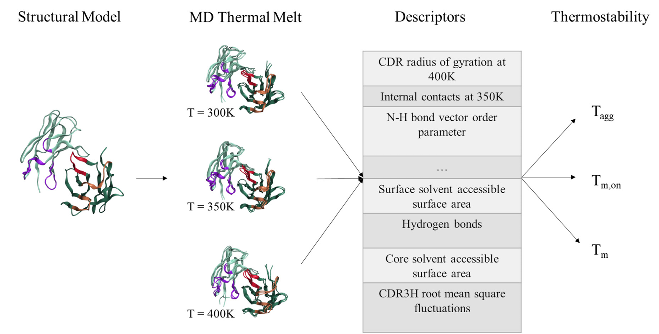
用到的描述符信息如下图所示:
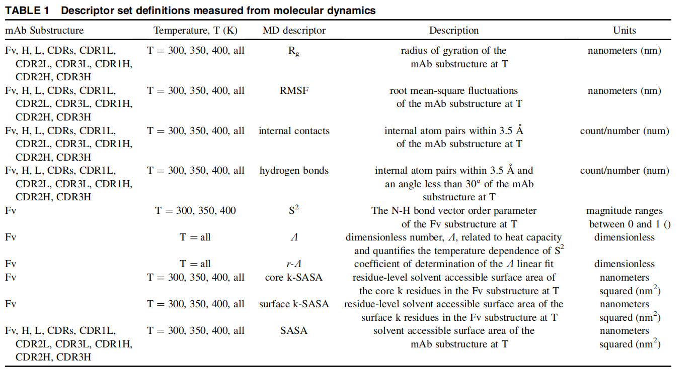
所有描述符的均值和标准差在20ns的平衡后以10ps的间隔计算。
对描述符进行筛选:
机器学习使用了8种常用方法:线性回归、弹性网络、支持向量机、k近邻、决策树、随机森林、adaboost和xgboost。最佳模型为:
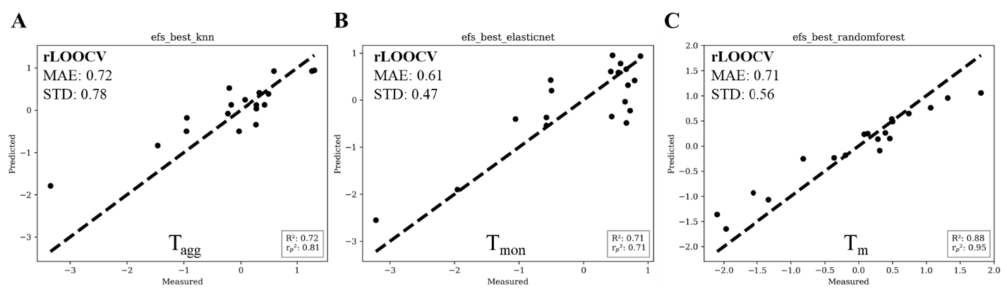
用于熔体温度预测的抗体Fv区结构,PDB格式。
输出文件名,包含Tm,on、Tm及Tagg预测值,CSV格式,默认为results.csv。
results.csv文件,包含如下信息:
| 列名 | 说明 |
|---|---|
| Name | 结构名称 |
| gyr_cdrs_Rg_std_350 | 温度350K时,CDR区域回转半径的标准差 |
| bonds_contacts_std_350 | 温度350K时,内部接触的标准差 |
| rmsf_cdrl1_std_350 | 温度350K时,CDRL1区域的RMSF标准差 |
| rmsf_cdrs_mu_400 | 温度400K时,CDR区域的RMSF平均值 |
| gyr_cdrs_Rg_std_400 | 温度400K时,CDR区域回转半径的标准差 |
| all-temp_lamda_b=25_eq=20 | lamda参数,与热容(heat capacity)相关,用于量化骨架结构N-H键矢量序参数(S²) 的温度依赖性 |
| all-temp-sasa_core_mean_k=20_eq=20 | 所有温度下,核心SASA的平均值 |
| all-temp-sasa_core_std_k=20_eq=20 | 所有温度下,核心SASA的标准差 |
| r-lamda_b=2.5_eq=20 | lamda参数的线性拟合决定系数 |
| Tm | 预测得到的Tm值 |
| Tagg | 预测得到的Tagg值 |
| Tmonset | 预测得到的Tm,on值 |
This module predicts the antibody melting onset temperature (Tm,on), melting temperature (Tm), and aggregation temperature (Tagg).
It is implemented based on the AbMelt model, which performs molecular dynamics (MD) simulations at three temperatures (300 K, 350 K, and 400 K) to generate structural ensembles corresponding to different stages of experimental thermal stability measurements.
AbMelt simulates the intrinsic flexibility of homologous antibody structures and learns relevant descriptors to predict corresponding melting temperatures.
The workflow of AbMelt is illustrated below:

Descriptor information used in the model is shown below:

All descriptor means and standard deviations are calculated over 20 ns of equilibrated trajectories, sampled at 10 ps intervals.
Descriptor selection was performed as follows:
Eight common machine-learning methods were evaluated:
Linear Regression, Elastic Net, Support Vector Machine, k-Nearest Neighbors, Decision Tree, Random Forest, AdaBoost, and XGBoost.
The best-performing models are shown below:

The antibody Fv-region structure used for melting temperature prediction, in PDB format.
Name of the output CSV file containing predicted Tm,on, Tm, and Tagg values.
Default: results.csv.
The file results.csv is generated, containing:
| Column Name | Description |
|---|---|
| Name | Structure name |
| gyr_cdrs_Rg_std_350 | Standard deviation of the radius of gyration (Rg) of the CDR regions at 350 K |
| bonds_contacts_std_350 | Standard deviation of internal contacts at 350 K |
| rmsf_cdrl1_std_350 | Standard deviation of RMSF for the CDRL1 region at 350 K |
| rmsf_cdrs_mu_400 | Mean RMSF of the CDR regions at 400 K |
| gyr_cdrs_Rg_std_400 | Standard deviation of the radius of gyration (Rg) of the CDR regions at 400 K |
| all-temp_lamda_b=25_eq=20 | Lambda parameter related to heat capacity, used to quantify the temperature dependence of the backbone N–H bond vector order parameter (S²) |
| all-temp-sasa_core_mean_k=20_eq=20 | Mean core SASA across all temperatures |
| all-temp-sasa_core_std_k=20_eq=20 | Standard deviation of core SASA across all temperatures |
| r-lamda_b=2.5_eq=20 | Coefficient of determination (R²) from the linear fit of the lambda parameter |
| Tm | Predicted melting temperature ™ |
| Tagg | Predicted aggregation temperature (Tagg) |
| Tmonset | Predicted onset melting temperature (Tm,onset) |
进行多肽(含环肽)的从头生成、性质计算与分析、格式转换等,支持非天然氨基酸。模块基于p2smi工具包实现。
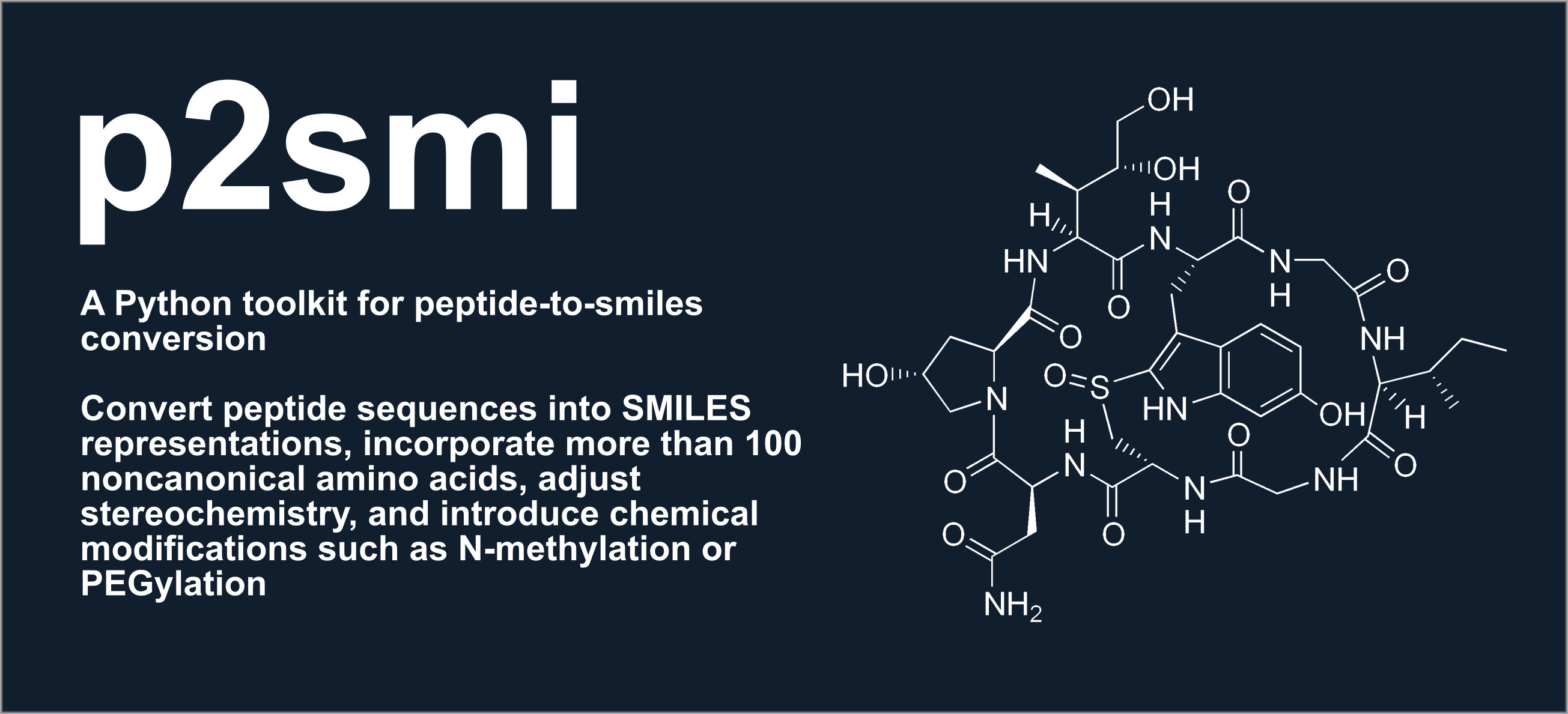
能够自动生成肽序列、将肽序列转换为 SMILES 字符串(支持环化结构和非天然氨基酸),并计算多种分子性质。此外,还提供修饰功能(如N-甲基化、PEG化)、合成可行性评估。
主要功能:
非标准氨基酸信息表(共411个):
| Name | Code | Formula | MolWeight | SMILES |
|---|---|---|---|---|
| Phenylglycine | PG | C8H9NO2 | 151.063328528 | N[C@@H](c1ccccc1)C(=O)O |
| 4-methoxy-Phenylalanine | 0A1 | C10H13NO3 | 195.089543276 | N[C@@H](Cc1ccc(OC)cc1)C(=O)O |
| … |
详细列表见附录。
根据自定义约束条件生成随机多肽序列。
生成的多肽序列数量,默认为10,最大为10000。
多肽序列最小长度,默认为10。
多肽序列最大长度,默认为20,最大长度为150。
每条多肽序列中的非天然氨基酸(NCAA, Non-Canonical Amino Acids)占比,默认为0.1(10%),数值范围为0.0 ~ 1.0(0%~100%)。
每条多肽序列中的D型氨基酸占比,默认为0.1(10%),数值范围为0.0 ~ 1.0(0%~100%)。
设置环肽的环化类型,可多选。all表示选择所有环肽类型,都不选时,则生成线性肽(默认为都不选)。
支持的环化类型如下:
| 标签(Tag) | 类型(Type) | 描述(Description) |
|---|---|---|
SS |
二硫键(Disulfide) | 半胱氨酸之间形成二硫键 |
HT |
头尾环化(Head-to-tail) | 在 N 端与 C 端之间(形成酰胺键) |
SCSC |
侧链–侧链(Sidechain–Sidechain) | 侧链之间成环(形成缩肽-酯键) |
SCNT |
侧链–N 端(Sidechain–N-Terminus) | 侧链与 N 末端成环(形成酰胺键) |
SCCT |
侧链–C 端(Sidechain–C-Terminus) | 侧链与 C 末端成环 |
生成的多肽序列文件,FASTA格式,默认为peptides.fasta。
将FASTA格式的肽序列转换为SMILES格式,环肽需指定环化类型。
多肽序列文件,FASTA格式。
注意:
大括号+非标准氨基酸Code表示 (例如:羟脯氨酸表示为{Hyp},常用非标准氨基酸Code请见附录列表。Cyclization Types)标注在序列名称中(用|与名称分隔)示例如下:
>seq_1
AVRENmV
>seq_2|SCCT
PyWT{DMEG}{0BN}IKaYI{TFG3}RWtNQ{I2M}
>seq_3|SCNT
KI{D6MW}E{AHP}iiARCKE{MEN}
序列seq_1是线性肽,由标准氨基酸和D型氨基酸m组成;seq_2是环肽,环化类型是SCCT,由标准氨基酸、D型氨基酸、非标准氨基酸组成;seq_3是环肽,环化类型是SCNT,由标准氨基酸、D型氨基酸、非标准氨基酸组成。
转换后的SMILES字符串,文本格式,每行一个。默认为peptides.smi。
转换前后对应的信息文件,CSV格式,默认为peptides.csv。
计算多肽的分子性质,包括:分子量(MW)、拓扑极性表面积(TPSA)、logP、氢键供体/受体、可旋转键数、环数量、Csp3 比例、重原子数、形式电荷、分子式,以及 Lipinski 规则评估等。
进行格式转换的多肽,支持两种格式:多肽序列文件(FASTA格式),或者多肽SMILES(文本格式,每行放置一个SMILES字符串)。
多肽的分子性质计算结果,CSV格式,默认为peptide_props.csv。
评估肽序列的可合成性,例如:N/Q 是否位于 N 端、Gly/Pro 模体、半胱氨酸数量、疏水性、总体电荷等。注意:目前仅支持天然氨基酸
多肽序列文件,FASTA格式。仅支持天然氨基酸的多肽。
可合成性评估结果,CSV格式,默认为synthesis_report.csv。
Generation模式,输出多肽序列FASTA文件,示例如下:
>seq_1|HT
{FLA}dAVREN{6CL}mV
>seq_2|SCCT
PyWT{DMEG}{0BN}IKaYI{TFG3}RWtNQ{I2M}
>seq_3|SCNT
KI{D6MW}E{AHP}iiARCKE{MEN}
>seq_4|HT
YlCP{YCM}yR{ESC}EiD{DDAB}HYSY{LMQ}GT
>seq_5|HT
{ORN}{AA4}TQAqP{CSA}YKI{DTTQ}aVvH
大括号+非标准氨基酸Code表示 (例如:羟脯氨酸表示为{Hyp}),常用非标准氨基酸Code请见附录列表。Cyclization Types)标注在序列名称中(用|与名称分隔)Format模式下,输出CSV文件和SMILES文件,CSV文件包含信息如下:
| 字段名称 | 示例 | 说明 |
|---|---|---|
| Name | seq_1 | 多肽序列名称 |
| Type | HT | 环肽的环化类型,线性肽为空值 |
| Sequence | FALPciA{DQ36}S{ONL}MV{TTQ}RS | 多肽序列 |
| SMILES | N3{C@@H}(Cc1ccccc1)C(=O) | 转换后的SMILES字符串 |
Property模式,输出CSV文件,包含信息如下:
| 字段名称 | 示例 | 说明 |
|---|---|---|
| Formula(分子式) | C49H80F3N15O17S | 分子的元素组成 |
| Molecular weight(分子量) | 1240.33 | 分子整体质量,单位道尔顿 |
| logP(脂溶性) | -4.76 | 越低越亲水,该分子极度亲水 |
| TPSA(拓扑极性表面积) | 516.33 | 反映极性强弱,越高越不易透膜 |
| H-bond donors(氢键供体) | 16 | 可提供氢键的基团数量 |
| H-bond acceptors(氢键受体) | 17 | 可接受氢键的基团数量 |
| Rotatable bonds(可旋转键) | 21 | 分子柔性的衡量指标 |
| Rings(环数量) | 1 | 分子内部的环结构数 |
| Fraction Csp3(Csp³ 碳比例) | 0.694 | 反映三维度的比例(越高越立体) |
| Heavy atoms(重原子数) | 85 | 除氢以外的原子数量 |
| Formal charge(形式电荷) | 0 | 分子整体电中性 |
| Lipinski pass(Lipinski 规则) | false | 不符合口服小分子规则(很正常,因其为大分子肽) |
Feasibility of Synthesis模式,输出CSV文件,包含信息如下:
| 字段名称 | 示例 | 说明 |
|---|---|---|
| Name | seq_1 | 多肽序列名称 |
| Result | FAIL | 合成可行性评价,PASS表示好,FAIL表示差 |
| Description | Failed charge: need 1 charged residue every 5 residues | 合成可行性差的原因说明 |
| Sequence | FALPciA{DQ36}S{ONL}MV{TTQ}RS | 多肽序列 |
非标准氨基酸信息表
| Name | Code | Formula | MolWeight | SMILES |
|---|---|---|---|---|
| Phenylglycine | PG | C8H9NO2 | 151.063328528 | N[C@@H](c1ccccc1)C(=O)O |
| 4-methoxy-Phenylalanine | 0A1 | C10H13NO3 | 195.089543276 | N[C@@H](Cc1ccc(OC)cc1)C(=O)O |
| 7-hydroxy-l-tryptophan | 0AF | C11H12N2O3 | 220.084792244 | N[C@@H](Cc1c[nH]c2c1cccc2O)C(=O)O |
| 4-carbamimidoyl-l-phenylalanine | 0BN | C10H13N3O2 | 207.100776656 | N[C@@H](Cc1ccc(cc1)C(=N)N)C(=O)O |
| 4-chloro-Phenylalanine | 4CP | C9H10ClNO2 | 199.04000624 | N[C@@H](Cc1ccc(cc1)Cl)C(=O)O |
| 2-Allyl-glycine | 2AG | C7H11NO5 | 189.063722452 | N[C@@H](CCCC(C(=O)O)=O)C(=O)O |
| 3-methyl-aspartic-acid | 2AS | C5H9NO4 | 147.053157768 | N[C@H]([C@H](C)(C(=O)O))C(=O)O |
| s-(difluoromethyl)-homocysteine | 2FM | C5H9F2NO2S | 185.032205968 | N[C@@H](CCSC(F)F)C(=O)O |
| 2-fluoro-l-histidine | 2HF | C6H12FN3O2 | 177.091354844 | N[C@@H](C[C@@H]1CN[C@@H](N1)F)C(=O)O |
| 2-fluoro-l-histidine(1) | 2HF1 | C6H8FN3O2 | 173.060054716 | N[C@@H](Cc1cnc(F)N1)C(=O)O |
| 2-fluoro-l-histidine(2) | 2HF2 | C6H8FN3O2 | 173.060054716 | N[C@@H](Cc1c[nH]c(n1)F)C(=O)O |
| l-2-amino-6-methylene-pimelic-acid | 2NP | C8H13NO4 | 187.084457896 | N[C@@H](CCCC(=C)C(=O)O)C(=O)O |
| 3-(4H-thieno[3,2-b]pyrrol-6-yl)-L-alanine | 32T | C9H10N2O2S | 210.04629856 | N[C@H](Cc1c[nH]c2c1scc2)C(=O)O |
| 3-cyano-phenylalanine | 3CF | C10H10N2O2 | 190.07422756 | N[C@@H](Cc1cccc(C#N)c1)C(=O)O |
| (2s)-amino(3,5-dihydroxyphenyl)-ethanoic-acid | 3FG | C8H9NO4 | 183.053157768 | N[C@@H](c1cc(O)cc(c1)O)C(=O)O |
| 4-hydroxy-glutamic-acid | 3GL | C5H9NO5 | 163.048072388 | N[C@@H](C[C@@H](C(=O)O)O)C(=O)O |
| 3-Chloro-tyrosine | 3MY | C9H10ClNO3 | 215.03492086 | N[C@H](Cc1ccc(c(c1)Cl)O)C(=O)O |
| 4-Bromo-phenylalanine | 4BF | C9H10BrNO2 | 242.98949066 | N[C@@H](Cc1ccc(cc1)Br)C(=O)O |
| 4-cyano-phenylalanine | 4CF | C10H10N2O2 | 190.07422756 | N[C@@H](Cc1ccc(cc1)C#N)C(=O)O |
| nitrilo-l-methionine | 4CY | C5H8N2O2S | 160.030648496 | N[C@@H](CCSC#N)C(=O)O |
| 4-fluoro-tryptophan | 4FW | C11H11FN2O2 | 222.080455812 | N[C@@H](Cc1c[nH]c2c1c(F)ccc2)C(=O)O |
| 4-hydroxymethyl-phenylalanine | 4HMP | C10H13NO3 | 195.089543276 | N[C@@H](Cc1ccc(CO)cc1)C(=O)O |
| 4-hydroxy-tryptophan | 4HT | C11H12N2O3 | 220.084792244 | N[C@@H](Cc1c[nH]c2c1c(O)ccc2)C(=O)O |
| 4-amino-l-tryptophan | 4IN | C11H13N3O2 | 219.100776656 | N[C@@H](Cc1c[nH]c2c1c(N)ccc2)C(=O)O |
| 4-methyl-phenylalanine | 4PH | C10H13NO2 | 179.094628656 | N[C@@H](Cc1ccc(cc1)C)C(=O)O |
| 6-carboxylysine | 6CL | C7H14N2O4 | 190.095356928 | N[C@@H](CCC[C@H](C(=O)O)N)C(=O)O |
| 6-chloro-l-tryptophan | 6CW | C11H11ClN2O2 | 238.050905272 | N[C@@H](Cc1c[nH]c2c1ccc(c2)Cl)C(=O)O |
| 2-amino-5-hydroxypentanoic-acid | AA4 | C5H11NO3 | 133.073893212 | N[C@@H](CCCO)C(=O)O |
| 2-Aminobutyric-acid | ABA | C4H9NO2 | 103.063328528 | N[C@@H](CC)C(=O)O |
| cis-amiclenomycin | ACZ | C10H16N2O2 | 196.121177752 | N[C@@H](CC[C@@H]1C=C[C@@H](C=C1)N)C(=O)O |
| Adamanthane | ADAM | C13H21NO2 | 223.157228912 | N[C@@H](C[C@]12C[C@H]3C[C@@H](C2)C[C@@H](C1)C3)C(=O)O |
| 5-methyl-arginine | AGM | C7H16N4O2 | 188.127325752 | N[C@@H](CC[C@H](C)NC(=N)N)C(=O)O |
| beta-hydroxyasparagine | AHB | C4H8N2O4 | 148.048406736 | N[C@@H]([C@@H](C(=O)N)O)C(=O)O |
| 2-Aminoheptanoic-acid | AHP | C7H15NO2 | 145.11027872 | N[C@@H](CCCCC)C(=O)O |
| 3-cyclohexyl-alanine | ALC | C9H17NO2 | 171.125928784 | N[C@@H](CC1CCCCC1)C(=O)O |
| 1-Naphthyl-alanine | ALN | C13H13NO2 | 215.094628656 | N[C@@H](Cc1cccc2c1cccc2)C(=O)O |
| Allo-threonine | ALO | C4H9NO3 | 119.058243148 | N[C@@H]([C@H](C)O)C(=O)O |
| 3-(9-anthryl)-alanine | ANTH | C17H15NO2 | 265.11027872 | N[C@@H](Cc1c2ccccc2cc2c1cccc2)C(=O)O |
| 3-Methyl-phenylalanine | APD | C10H13NO2 | 179.094628656 | N[C@@H](Cc1cccc(c1)C)C(=O)O |
| m-amidinophenyl-3-alanine | APM | C10H13N3O2 | 207.100776656 | N[C@@H](Cc1cccc(c1)C(=N)N)C(=O)O |
| c-gamma-hydroxy-arginine | ARO | C6H14N4O3 | 190.106590308 | N[C@@H](C[C@@H](O)CN=C(N)N)C(=O)O |
| (2r)-2-amino-4-oxobutanoic-acid | AS2 | C4H7NO3 | 117.042593084 | N[C@@H](CC=O)C(=O)O |
| azido-alanine | AZDA | C3H7N4O2+ | 131.05635188409 | N[C@@H](CN=[N+]=N)C(=O)O |
| Phenylserine | BB8 | C9H11NO3 | 181.073893212 | N[C@@H]([C@@H](O)c1ccccc1)C(=O)O |
| benzylcysteine | BCS | C10H13NO2S | 211.066699656 | N[C@@H](CSCc1ccccc1)C(=O)O |
| beta-hydroxyaspartic-acid | BHD | C4H7NO5 | 149.032422324 | N[C@@H]([C@H](O)C(=O)O)C(=O)O |
| 4,4-biphenylalanine | BIF | C15H15NO2 | 241.11027872 | N[C@@H](Cc1ccc(cc1)c1ccccc1)C(=O)O |
| 5-bromo-l-isoleucine | BIU | C6H12BrNO2 | 209.005140724 | N[C@@H]([C@@H](C)CCBr)C(=O)O |
| 3-(3-benzothienyl)-alanine | BTH3 | C11H11NO2S | 221.051049592 | N[C@@H](Cc1csc2c1cccc2)C(=O)O |
| 6-bromo-tryptophan | BTR | C11H11BrN2O2 | 282.000389692 | N[C@@H](Cc1c[nH]c2c1ccc(c2)Br)C(=O)O |
| Tertleucine | BUG | C6H13NO2 | 131.094628656 | N[C@@H](C(C)(C)C)C(=O)O |
| 3-chloro-l-alanine | C2N | C3H6ClNO2 | 123.008706112 | N[C@@H](CCl)C(=O)O |
| canaline | CAN | C4H10N2O3 | 134.06914218 | N[C@@H](CCON)C(=O)O |
| carboxymethylated-cysteine | CCS | C5H9NO4S | 179.025228768 | N[C@@H](CSCC(=O)O)C(=O)O |
| Cyclohexylglycine | CHG | C8H15NO2 | 157.11027872 | N[C@@H](C1CCCCC1)C(=O)O |
| 3-chloro-4-hydroxy-phenylglycine | CHP | C8H8ClNO3 | 201.019270796 | N[C@@H](c1ccc(c(c1)Cl)O)C(=O)O |
| Citrulline | CIR | C6H13N3O3 | 175.095691276 | N[C@@H](CCC[NH]C(=O)N)C(=O)O |
| 2-cyano-phenylalanine | CNP2 | C10H10N2O2 | 190.07422756 | N[C@@H](Cc1ccccc1C#N)C(=O)O |
| 2,4-dichloro-phenylalanine | CP24 | C9H9Cl2NO2 | 233.001033888 | N[C@@H](Cc1ccc(cc1Cl)Cl)C(=O)O |
| 3,4-dichloro-phenylalanine | CP34 | C9H9Cl2NO2 | 233.001033888 | N[C@@H](Cc1ccc(c(c1)Cl)Cl)C(=O)O |
| 3-Cyclopentyl-alanine | CPA3 | C8H15NO2 | 157.11027872 | N[C@@H](CC1CCCC1)C(=O)O |
| 2-Chloro-phenylglycine | CPG2 | C8H8ClNO2 | 185.024356176 | N[C@@H](c1ccccc1Cl)C(=O)O |
| 3-Chloro-phenylglycine | CPG3 | C8H8ClNO2 | 185.024356176 | N[C@@H](c1cccc(c1)Cl)C(=O)O |
| 4-Chloro-phenylglycine | CPG4 | C8H8ClNO2 | 185.024356176 | N[C@@H](c1ccc(cc1)Cl)C(=O)O |
| 2-chloro-Phenylalanine | CPH2 | C9H10ClNO2 | 199.04000624 | N[C@@H](Cc1ccccc1Cl)C(=O)O |
| s-acetonylcysteine | CSA | C6H11NO3S | 177.045964212 | N[C@@H](CSCC(=O)C)C(=O)O |
| Selenocysteine | CSE | C3H7NO2Se | 168.964199764 | N[C@@H](C[SeH])C(=O)O |
| 7-chloro-tryptophan | CTE | C11H11ClN2O2 | 238.050905272 | N[C@@H](Cc1cNc2c1cccc2Cl)C(=O)O |
| 4-chloro-threonine | CTH | C4H8ClNO3 | 153.019270796 | N[C@@H]([C@H](O)CCl)C(=O)O |
| 4-Hydroxy-phenylglycine | D4P | C8H9NO3 | 167.058243148 | N[C@@H](c1ccc(cc1)O)C(=O)O |
| Diaminobutyric-acid | DAB | C4H10N2O2 | 118.07422756 | N[C@@H](CCN)C(=O)O |
| 3,4-Dihydroxy-phenylalanine | DAH | C9H11NO4 | 197.068807832 | N[C@@H](Cc1ccc(c(c1)O)O)C(=O)O |
| 3,5-dibromotyrosine | DBY | C9H9Br2NO3 | 336.894917348 | N[C@@H](Cc1cc(Br)c(c(c1)Br)O)C(=O)O |
| 3,3-dihydroxy-alanine | DDZ | C3H7NO4 | 121.037507704 | N[C@@H](C(O)O)C(=O)O |
| Diethylalanine | DILE | C7H15NO2 | 145.11027872 | N[C@@H](C(CC)CC)C(=O)O |
| 3,3-diphenylalanine | DIPH | C15H15NO2 | 241.11027872 | N[C@@H]([C@H](c1ccccc1)c1ccccc1)C(=O)O |
| 3,3-dimethyl-aspartic-acid | DMK | C6H11NO4 | 161.068807832 | N[C@@H](C(C(=O)O)(C)C)C(=O)O |
| 3-ethyl-phenylalanine | DMP3 | C11H15NO2 | 193.11027872 | N[C@@H](Cc1cc(CC)ccc1)C(=O)O |
| 2,3-Diaminopropanoic-acid | DPP | C3H8N2O2 | 104.058577496 | N[C@@H](CN)C(=O)O |
| Ethionine | ESC | C6H13NO2S | 163.066699656 | N[C@@H](CCSCC)C(=O)O |
| 3,4-Difluoro-phenylalanine | F2F | C9H9F2NO2 | 201.060134968 | N[C@@H](Cc1ccc(c(c1)F)F)C(=O)O |
| 3-chloro-Phenylalanine | FCL | C9H10ClNO2 | 199.04000624 | N[C@@H](Cc1cccc(c1)Cl)C(=O)O |
| 4-Fluoro-glutamic-acid | FGA4 | C5H8FNO4 | 165.043735956 | N[C@@H](C[C@H](F)C(=O)O)C(=O)O |
| 2-amino-propanedioic-acid | FGL | C3H5NO4 | 119.02185764 | NC(C(=O)O)C(=O)O |
| Trifluoro-alanine | FLA | C3H4F3NO2 | 143.019413028 | N[C@@H](C(F)(F)F)C(=O)O |
| 2-Fluoro-phenylglycine | FPG2 | C8H8FNO2 | 169.053906716 | N[C@@H](c1ccccc1F)C(=O)O |
| 3-Fluoro-phenylglycine | FPG3 | C8H8FNO2 | 169.053906716 | N[C@@H](c1cccc(c1)F)C(=O)O |
| 4-Fluoro-phenylglycine | FPG4 | C8H8FNO2 | 169.053906716 | N[C@@H](c1ccc(cc1)F)C(=O)O |
| 2-Fluoro-Phenylalanine | FPH2 | C9H10FNO2 | 183.06955678 | N[C@@H](Cc1ccccc1F)C(=O)O |
| 3-Fluoro-Phenylalanine | FPH3 | C9H10FNO2 | 183.06955678 | N[C@@H](Cc1cccc(c1)F)C(=O)O |
| 6-fluoro-l-tryptophan | FT6 | C11H11FN2O2 | 222.080455812 | N[C@@H](Cc1cNc2c1ccc(c2)F)C(=O)O |
| 5-Fluoro-tryptophan | FTR | C11H11FN2O2 | 222.080455812 | N[C@@H](Cc1c[nH]c2c1cc(F)cc2)C(=O)O |
| (2-furyl)-alanine | FUA2 | C7H9NO3 | 155.058243148 | N[C@@H](Cc1ccco1)C(=O)O |
| 3-Fluoro-valine | FVAL | C5H10FNO2 | 135.06955678 | N[C@@H](C(F)(C)C)C(=O)O |
| 2-Amino-4-guanidinobutryric-acid | GBUT | C5H14N4O2 | 162.111675688 | N[C@@H](CCNC(N)N)C(=O)O |
| 2-Amino-3-guanidinopropionic-acid | GDPR | C4H12N4O2 | 148.096025624 | N[C@@H](CNC(N)N)C(=O)O |
| Canavanine | GGB | C5H12N4O3 | 176.090940244 | N[C@@H](CCON=C(N)N)C(=O)O |
| (2s,4s)-2,5-diamino-4-hydroxy-5-oxopentanoic-acid | GHG | C5H10N2O4 | 162.0640568 | N[C@@H](C[C@H](O)C(=O)N)C(=O)O |
| 5-o-methyl-glutamic-acid | GME | C6H11NO4 | 161.068807832 | N[C@@H](CCC(=O)OC)C(=O)O |
| homocysteine | HCS | C4H9NO2S | 135.035399528 | N[C@@H](CCS)C(=O)O |
| glutamine-hydroxamate | HGA | C5H10N2O4 | 162.0640568 | N[C@@H](CCC(=O)NO)C(=O)O |
| (2s)-2,8-diaminooctanoic-acid | HHK | C8H18N2O2 | 174.136827816 | N[C@@H](CCCCCCN)C(=O)O |
| 4-Hydroxy-L-isoleucine | HIL4 | C6H13NO3 | 147.089543276 | N[C@@H]([C@H]([C@@H](C)O)C)C(=O)O |
| (2s,3r)-2-amino-3-hydroxy-4-methylpentanoic-acid | HL2 | C6H13NO3 | 147.089543276 | N[C@@H]([C@H](O)C(C)C)C(=O)O |
| Homoleucine | HLEU | C7H15NO2 | 145.11027872 | N[C@@H](CCC(C)C)C(=O)O |
| beta-hydroxyleucine | HLU | C6H13NO3 | 147.089543276 | N[C@@H]([C@@H](O)C(C)C)C(=O)O |
| 4-amino-L-phenylalanine | HOX | C9H12N2O2 | 180.089877624 | N[C@@H](Cc1ccc(cc1)N)C(=O)O |
| Homophenylalanine | HPE | C10H13NO2 | 179.094628656 | N[C@@H](CCc1ccccc1)C(=O)O |
| 3-(8-hydroxyquinolin-3-yl)-l-alanine | HQA | C12H12N2O3 | 232.084792244 | N[C@@H](Cc1cnc2c(c1)cccc2O)C(=O)O |
| homoarginine | HRG | C7H18N4O2 | 190.142975816 | N[C@@H](CCCCNC(N)N)C(=O)O |
| 5-Hydroxy-tryptophan | HRP | C11H12N2O3 | 220.084792244 | N[C@@H](Cc1cNc2c1cc(O)cc2)C(=O)O |
| homoserine | HSER | C4H9NO3 | 119.058243148 | N[C@@H](CCO)C(=O)O |
| beta-hydroxy-tryptophane | HTR | C11H12N2O3 | 220.084792244 | N[C@@H]([C@H](c1c[nH]c2c1cccc2)O)C(=O)O |
| 3-hydroxy-l-valine | HVA | C5H11NO3 | 133.073893212 | N[C@@H](C(O)(C)C)C(=O)O |
| 3-methyl-l-alloisoleucine | I2M | C7H15NO2 | 145.11027872 | N[C@@H](C(CC)(C)C)C(=O)O |
| alpha-amino-2-indanacetic-acid | IGL | C11H13NO2 | 191.094628656 | N[C@@H](C1Cc2c(C1)cccc2)C(=O)O |
| Allo-Isoleucine | IIL | C6H13NO2 | 131.094628656 | N[C@@H]([C@@H](CC)C)C(=O)O |
| 4,5-dihydroxy-isoleucine | ILX | C6H13NO4 | 163.084457896 | N[C@@H]([C@H]([C@H](CO)O)C)C(=O)O |
| 3-iodo-tyrosine | IYR | C9H10INO3 | 306.97054117999994 | N[C@@H](Cc1ccc(c(c1)I)O)C(=O)O |
| kynurenine | KYN | C10H12N2O3 | 208.084792244 | N[C@@H](CC(=O)c1ccccc1N)C(=O)O |
| 6-hydroxy-l-norleucine | LDO | C6H13NO3 | 147.089543276 | N[C@@H](CCCCO)C(=O)O |
| Penicillamine | LE1 | C5H11NO2S | 149.051049592 | N[C@@H](C(S)(C)C)C(=O)O |
| (4r)-5-oxo-l-leucine | LED | C6H11NO3 | 145.073893212 | N[C@@H](C[C@@H](C)C=O)C(=O)O |
| (4s)-5-fluoro-l-leucine | LEF | C6H12FNO2 | 149.085206844 | N[C@@H](C[C@H](C)CF)C(=O)O |
| (3r)-3-methyl-l-glutamic-acid | LME | C6H11NO4 | 161.068807832 | N[C@@H]([C@H](C)CC(=O)O)C(=O)O |
| 3-methyl-l-glutamine | LMQ | C6H12N2O3 | 160.084792244 | N[C@@H]([C@@H](C)CC(N)=O)C(=O)O |
| vinylglycine | LVG | C4H7NO2 | 101.047678464 | N[C@@H](C=C)C(=O)O |
| 4-oxo-l-valine | LVN | C5H9NO3 | 131.058243148 | N[C@@H]([C@H](C)C=O)C(=O)O |
| 3,3-dimethyl-methionine-sulfoxide | M2S | C7H15NO3S | 193.07726434 | N[C@@H](C(C)(C)C[S@@](C)=O)C(=O)O |
| hydroxy-l-methionine | ME0 | C5H11NO3S | 165.045964212 | N[C@@H](CCSCO)C(=O)O |
| (3s)-3-methyl-l-glutamic-acid | MEG | C6H11NO4 | 161.068807832 | N[C@@H]([C@@H](C)CC(=O)O)C(=O)O |
| n-methyl-asparagine | MEN | C5H10N2O3 | 146.06914218 | N[C@@H](CC(=O)NC)C(=O)O |
| n5-methyl-glutamine | MEQ | C6H12N2O3 | 160.084792244 | N[C@@H](CCC(=O)NC)C(=O)O |
| s-oxymethionine | MHO | C5H11NO3S | 165.045964212 | N[C@@H](CC[S@](=O)C)C(=O)O |
| 5-Methoxy-tryptophan | MOT5 | C12H14N2O3 | 234.100442308 | N[C@@H](Cc1cNc2ccc(OC)cc12)C(=O)O |
| 3,4-Dimethyl-phenylalanine | MP34 | C11H15NO2 | 193.11027872 | N[C@@H](Cc1ccc(c(c1)C)C)C(=O)O |
| 2-Methyl-phenylalanine | MPH2 | C10H13NO2 | 179.094628656 | N[C@@H](Cc1ccccc1C)C(=O)O |
| 5-Methyl-tryptophan | MTR5 | C12H14N2O2 | 218.105527688 | N[C@@H](Cc1cNc2ccc(C)cc12)C(=O)O |
| 6-Methyl-tryptophan | MTR6 | C12H14N2O2 | 218.105527688 | N[C@@H](Cc1cNc2c1ccc(c2)C)C(=O)O |
| m-Tyrosine | MTY | C9H11NO3 | 181.073893212 | N[C@@H](Cc1cccc(c1)O)C(=O)O |
| 2-Naphthyl-alanine | NAL | C13H13NO2 | 215.094628656 | N[C@@H](Cc1ccc2c(c1)cccc2)C(=O)O |
| 5-hydroxy-1-naphthalene | NAO1 | C13H13NO3 | 231.089543276 | N[C@@H](Cc1cccc2c1cc(O)cc2)C(=O)O |
| 6-hydroxy-2-naphthalene | NAO2 | C13H13NO3 | 231.089543276 | N[C@@H](Cc1ccc2c(c1)cc(cc2)O)C(=O)O |
| meta-nitro-tyrosine | NIY | C9H10N2O5 | 226.05897142 | N[C@@H](Cc1ccc(c(c1)N(=O)=O)O)C(=O)O |
| Norleucine | NLE | C6H13NO2 | 131.094628656 | N[C@@H](CCCC)C(=O)O |
| Norvaline | NVA | C5H11NO2 | 117.078978592 | N[C@@H](CCC)C(=O)O |
| o-acetylserine | OAS | C5H9NO4 | 147.053157768 | N[C@@H](COC(=O)C)C(=O)O |
| (2s)-2-amino-4,4-difluorobutanoic-acid | OBF | C4H7F2NO2 | 139.044484904 | N[C@@H](CC(F)F)C(=O)O |
| s-(2-hydroxyethyl)-l-cysteine | OCY | C5H11NO3S | 165.045964212 | N[C@@H](CSCCO)C(=O)O |
| o-methyl-l-threonine | OLT | C5H11NO3 | 133.073893212 | N[C@@H]([C@H](OC)C)C(=O)O |
| Methionine-sulfone | OMT | C5H11NO4S | 181.040878832 | N[C@@H](CCS(=O)(=O)C)C(=O)O |
| (betar)-beta-hydroxy-l-tyrosine | OMX | C9H11NO4 | 197.068807832 | N[C@@H]([C@@H](c1ccc(cc1)O)O)C(=O)O |
| (betar)-3-chloro-beta-hydroxy-l-tyrosine | OMY | C9H10ClNO4 | 231.02983548 | N[C@@H]([C@@H](c1ccc(c(c1)Cl)O)O)C(=O)O |
| 5-oxo-l-norleucine | ONL | C6H11NO3 | 145.073893212 | N[C@@H](CCC(=O)C)C(=O)O |
| Ornithine | ORN | C5H12N2O2 | 132.089877624 | N[C@@H](CCCN)C(=O)O |
| o-Tyrosine | OTYR | C9H11NO3 | 181.073893212 | N[C@@H](Cc1ccccc1O)C(=O)O |
| 4-benzoyl-phenylalanine | PBF | C16H15NO3 | 269.10519334 | N[C@@H](Cc1ccc(cc1)C(=O)c1ccccc1)C(=O)O |
| pentafluoro-phenylalanine | PF5 | C9H6F5NO2 | 255.031869532 | N[C@@H](Cc1c(F)c(F)c(c(c1F)F)F)C(=O)O |
| 4-Fluoro-Phenylalanine | PFF | C9H10FNO2 | 183.06955678 | N[C@@H](Cc1ccc(cc1)F)C(=O)O |
| 4-Iodo-Phenylalanine | PHI | C9H10INO2 | 290.97562656 | N[C@@H](Cc1ccc(cc1)I)C(=O)O |
| 4-Nitro-phenylalanine | PPN | C9H10N2O4 | 210.0640568 | N[C@@H](Cc1ccc(cc1)N(=O)=O)C(=O)O |
| phosphotyrosine | PTR | C9H12NO6P | 261.04022373400005 | N[C@@H](Cc1ccc(cc1)OP(=O)(O)O)C(=O)O |
| 3-(2-Pyridyl)-alanine | PYR2 | C8H10N2O2 | 166.07422756 | N[C@@H](Cc1ccccn1)C(=O)O |
| 3-(3-Pyridyl)-alanine | PYR3 | C8H10N2O2 | 166.07422756 | N[C@@H](Cc1cccnc1)C(=O)O |
| 3-(4-Pyridyl)-alanine | PYR4 | C8H10N2O2 | 166.07422756 | N[C@@H](Cc1ccncc1)C(=O)O |
| 3-(1-Pyrazolyl)-alanine | PYZ1 | C6H9N3O2 | 155.069476528 | N[C@@H](Cn1cccn1)C(=O)O |
| 3-(2-Quinolyl)-alanine | QU32 | C12H12N2O2 | 216.089877624 | N[C@@H](Cc1ccc2c(n1)cccc2)C(=O)O |
| 3-(3-quinolyl)-alanine | QU33 | C12H12N2O2 | 216.089877624 | N[C@@H](Cc1cnc2c(c1)cccc2)C(=O)O |
| 3-(4-quinolyl)-alanine | QU34 | C12H12N2O2 | 216.089877624 | N[C@@H](Cc1ccnc2c1cccc2)C(=O)O |
| 3-(5-Quinolyl)-alanine | QU35 | C12H12N2O2 | 216.089877624 | N[C@@H](Cc1ccc2c(c1)nccc2)C(=O)O |
| 3-(6-Quinolyl)-alanine | QU36 | C12H12N2O2 | 216.089877624 | N[C@@H](Cc1ccc2c(c1)cncc2)C(=O)O |
| 3-(2-quinoxalyl)-alanine | QX32 | C11H11N3O2 | 217.085126592 | N[C@@H](Cc1cnc2c(n1)cccc2)C(=O)O |
| phosphoserine | SEP | C3H8NO6P | 185.008923606 | N[C@@H](COP(=O)(O)O)C(=O)O |
| thialysine | SLZ | C5H12N2O2S | 164.061948624 | N[C@@H](CSCCN)C(=O)O |
| Methionine-sulfoxide | SME | C5H11NO3S | 165.045964212 | N[C@@H](CC[S@](=O)C)C(=O)O |
| Styrylalanine | STYA | C11H13NO2 | 191.094628656 | N[C@@H](CC=Cc1ccccc1)C(=O)O |
| 2s,4r-4-methylglutamate | SYM | C6H11NO4 | 161.068807832 | N[C@@H](C[C@H](C(=O)O)C)C(=O)O |
| 4-tert-butyl-phenylalanine | TBP4 | C13H19NO2 | 221.141578848 | N[C@@H](Cc1ccc(cc1)C(C)(C)C)C(=O)O |
| 3-(2-Tetrazolyl)-alanine | TEZA | C4H7N5O2 | 157.059974464 | N[C@@H](Cn1nncn1)C(=O)O |
| 2-(Trifluoromethyl)-phenylglycine | TFG2 | C9H8F3NO2 | 219.050713156 | N[C@@H](c1ccccc1C(F)(F)F)C(=O)O |
| 3-(Trifluoromethyl)-phenylglycine | TFG3 | C9H8F3NO2 | 219.050713156 | N[C@@H](c1cccc(c1)C(F)(F)F)C(=O)O |
| 4-(Trifluoromethyl)-phenylglycine | TFG4 | C9H8F3NO2 | 219.050713156 | N[C@@H](c1ccc(cc1)C(F)(F)F)C(=O)O |
| 5,5,5-Trifluoro-leucine | TFLE | C6H10F3NO2 | 185.06636322 | N[C@@H](C[C@@H](C(F)(F)F)C)C(=O)O |
| 2-(Trifluoromethyl)-phenylalanine | TFP2 | C10H10F3NO2 | 233.06636322 | N[C@@H](Cc1ccccc1C(F)(F)F)C(=O)O |
| 3-(Trifluoromethyl)-phenylalanine | TFP3 | C10H10F3NO2 | 233.06636322 | N[C@@H](Cc1cccc(c1)C(F)(F)F)C(=O)O |
| 4-(Trifluoromethyl)-phenylalanine | TFP4 | C10H10F3NO2 | 233.06636322 | N[C@@H](Cc1ccc(cc1)C(F)(F)F)C(=O)O |
| 4-hydroxy-l-threonine | TH6 | C4H9NO4 | 135.053157768 | N[C@@H]([C@H](O)CO)C(=O)O |
| 3-(3-thienyl)-alanine | THA3 | C7H9NO2S | 171.035399528 | N[C@@H](Cc1cscc1)C(=O)O |
| 2-thienylglycine | THG2 | C6H7NO2S | 157.019749464 | N[C@@H](c1cccs1)C(=O)O |
| 3-thienylglycine | THG3 | C6H7NO2S | 157.019749464 | N[C@@H](c1cscc1)C(=O)O |
| Thio-citrulline | THIC | C6H13N3O2S | 191.072847656 | N[C@@H](CCCNC(=S)N)C(=O)O |
| 3-(2-thienyl)-alanine | TIH | C7H9NO2S | 171.035399528 | N[C@@H](Cc1cccs1)C(=O)O |
| phosphothreonine | TPO | C4H10NO6P | 199.02457367 | N[C@@H]([C@H](OP(=O)(O)O)C)C(=O)O |
| 2-hydroxy-tryptophan | TRO | C11H12N2O3 | 220.084792244 | N[C@@H](Cc1c(O)[nH]c2c1cccc2)C(=O)O |
| 6-hydroxy-tryptophan | TRX | C11H12N2O3 | 220.084792244 | N[C@@H](Cc1c[nH]c2c1ccc(c2)O)C(=O)O |
| 3-(1,2,4-Triazol-1-yl)-alanine | TRZ4 | C5H8N4O2 | 156.064725496 | N[C@@H](Cn1cncn1)C(=O)O |
| 6-amino-7-hydroxy-l-tryptophan | TTQ | C11H13N3O3 | 235.095691276 | N[C@@H](Cc1c[nH]c2c1ccc(c2O)N)C(=O)O |
| 3-Amino-L-tyrosine | TY2 | C9H12N2O3 | 196.084792244 | N[C@@H](Cc1ccc(c(c1)N)O)C(=O)O |
| 3,5-diiodotyrosine | TYI | C9H9I2NO3 | 432.8671891479999 | N[C@@H](Cc1cc(I)c(c(c1)I)O)C(=O)O |
| 3-amino-6-hydroxy-tyrosine | TYQ | C9H12N2O4 | 212.079706864 | N[C@@H](Cc1cc(N)c(cc1O)O)C(=O)O |
| (4-thiazolyl)-alanine | TZA4 | C6H8N2O2S | 172.030648496 | N[C@@H](Cc1cscn1)C(=O)O |
| 2-Aminoadipic-acid | UN1 | C6H11NO4 | 161.068807832 | N[C@@H](CCCC(=O)O)C(=O)O |
| Hydroxynorvaline | VAH | C5H11NO3 | 133.073893212 | N[C@@H]([C@H](O)CC)C(=O)O |
| 3,5-Difluoro-phenylalanine | WFP | C9H9F2NO2 | 201.060134968 | N[C@@H](Cc1cc(F)cc(c1)F)C(=O)O |
| cysteine-s-acetamide | YCM | C5H10N2O3S | 178.04121318 | N[C@@H](CSCC(=O)N)C(=O)O |
| 3-fluorotyrosine | YOF | C9H10FNO3 | 199.0644714 | N[C@@H](Cc1ccc(c(c1)F)O)C(=O)O |
| d-Phenylglycine | DPG | C8H9NO2 | 151.063328528 | N[C@H](c1ccccc1)C(=O)O |
| d-4-methoxy-Phenylalanine | D0A1 | C10H13NO3 | 195.089543276 | N[C@H](Cc1ccc(OC)cc1)C(=O)O |
| d-7-hydroxy-l-tryptophan | D0AF | C11H12N2O3 | 220.084792244 | N[C@H](Cc1c[nH]c2c1cccc2O)C(=O)O |
| d-4-carbamimidoyl-l-phenylalanine | D0BN | C10H13N3O2 | 207.100776656 | N[C@H](Cc1ccc(cc1)C(=N)N)C(=O)O |
| d-4-chloro-Phenylalanine | D200 | C9H10ClNO2 | 199.04000624 | N[C@H](Cc1ccc(cc1)Cl)C(=O)O |
| d-2-Allyl-glycine | D2AG | C7H11NO5 | 189.063722452 | N[C@H](CCCC(C(=O)O)=O)C(=O)O |
| d-3-methyl-aspartic-acid | D2AS | C5H9NO4 | 147.053157768 | N[C@@H]([C@H](C)(C(=O)O))C(=O)O |
| d-s-(difluoromethyl)-homocysteine | D2FM | C5H9F2NO2S | 185.032205968 | N[C@H](CCSC(F)F)C(=O)O |
| d-2-fluoro-l-histidine | D2HF | C6H12FN3O2 | 177.091354844 | N[C@H](C[C@@H]1CN[C@@H](N1)F)C(=O)O |
| d-2-fluoro-l-histidine(1) | D2H1 | C6H8FN3O2 | 173.060054716 | N[C@H](Cc1cnc(F)N1)C(=O)O |
| d-2-fluoro-l-histidine(2) | D2H2 | C6H8FN3O2 | 173.060054716 | N[C@H](Cc1c[nH]c(n1)F)C(=O)O |
| d-l-2-amino-6-methylene-pimelic-acid | D2NP | C8H13NO4 | 187.084457896 | N[C@H](CCCC(=C)C(=O)O)C(=O)O |
| d-3-(4H-thieno[3,2-b]pyrrol-6-yl)-L-alanine | D32T | C9H10N2O2S | 210.04629856 | N[C@@H](Cc1c[nH]c2c1scc2)C(=O)O |
| d-3-cyano-phenylalanine | D3CF | C10H10N2O2 | 190.07422756 | N[C@H](Cc1cccc(C#N)c1)C(=O)O |
| d-(2s)-amino(3,5-dihydroxyphenyl)-ethanoic-acid | D3FG | C8H9NO4 | 183.053157768 | N[C@H](c1cc(O)cc(c1)O)C(=O)O |
| d-4-hydroxy-glutamic-acid | D3GL | C5H9NO5 | 163.048072388 | N[C@H](C[C@@H](C(=O)O)O)C(=O)O |
| d-3-Chloro-tyrosine | D3MY | C9H10ClNO3 | 215.03492086 | N[C@@H](Cc1ccc(c(c1)Cl)O)C(=O)O |
| d-4-Bromo-phenylalanine | D4BF | C9H10BrNO2 | 242.98949066 | N[C@H](Cc1ccc(cc1)Br)C(=O)O |
| d-4-cyano-phenylalanine | D4CF | C10H10N2O2 | 190.07422756 | N[C@H](Cc1ccc(cc1)C#N)C(=O)O |
| d-nitrilo-l-methionine | D4CY | C5H8N2O2S | 160.030648496 | N[C@H](CCSC#N)C(=O)O |
| d-4-fluoro-tryptophan | D4FW | C11H11FN2O2 | 222.080455812 | N[C@H](Cc1c[nH]c2c1c(F)ccc2)C(=O)O |
| d-4-hydroxymethyl-phenylalanine | D4HZ | C10H13NO3 | 195.089543276 | N[C@H](Cc1ccc(CO)cc1)C(=O)O |
| d-4-hydroxy-tryptophan | D4HT | C11H12N2O3 | 220.084792244 | N[C@H](Cc1c[nH]c2c1c(O)ccc2)C(=O)O |
| d-4-amino-l-tryptophan | D4IN | C11H13N3O2 | 219.100776656 | N[C@H](Cc1c[nH]c2c1c(N)ccc2)C(=O)O |
| d-4-methyl-phenylalanine | D4PH | C10H13NO2 | 179.094628656 | N[C@H](Cc1ccc(cc1)C)C(=O)O |
| d-6-carboxylysine | D6CL | C7H14N2O4 | 190.095356928 | N[C@H](CCC[C@H](C(=O)O)N)C(=O)O |
| d-6-chloro-l-tryptophan | D6CW | C11H11ClN2O2 | 238.050905272 | N[C@H](Cc1c[nH]c2c1ccc(c2)Cl)C(=O)O |
| d-2-amino-5-hydroxypentanoic-acid | DAA4 | C5H11NO3 | 133.073893212 | N[C@H](CCCO)C(=O)O |
| d-2-Aminobutyric-acid | DABA | C4H9NO2 | 103.063328528 | N[C@H](CC)C(=O)O |
| d-cis-amiclenomycin | DACZ | C10H16N2O2 | 196.121177752 | N[C@H](CC[C@@H]1C=C[C@@H](C=C1)N)C(=O)O |
| d-Adamanthane | DADM | C13H21NO2 | 223.157228912 | N[C@H](C[C@]12C[C@H]3C[C@@H](C2)C[C@@H](C1)C3)C(=O)O |
| d-5-methyl-arginine | DAGM | C7H16N4O2 | 188.127325752 | N[C@H](CC[C@H](C)NC(=N)N)C(=O)O |
| d-beta-hydroxyasparagine | DAHB | C4H8N2O4 | 148.048406736 | N[C@H]([C@@H](C(=O)N)O)C(=O)O |
| d-2-Aminoheptanoic-acid | DAHP | C7H15NO2 | 145.11027872 | N[C@H](CCCCC)C(=O)O |
| d-3-cyclohexyl-alanine | DALC | C9H17NO2 | 171.125928784 | N[C@H](CC1CCCCC1)C(=O)O |
| d-1-Naphthyl-alanine | DALN | C13H13NO2 | 215.094628656 | N[C@H](Cc1cccc2c1cccc2)C(=O)O |
| d-Allo-threonine | DALO | C4H9NO3 | 119.058243148 | N[C@H]([C@H](C)O)C(=O)O |
| d-3-(9-anthryl)-alanine | DNTL | C17H15NO2 | 265.11027872 | N[C@H](Cc1c2ccccc2cc2c1cccc2)C(=O)O |
| d-3-Methyl-phenylalanine | DAPD | C10H13NO2 | 179.094628656 | N[C@H](Cc1cccc(c1)C)C(=O)O |
| d-m-amidinophenyl-3-alanine | DAPM | C10H13N3O2 | 207.100776656 | N[C@H](Cc1cccc(c1)C(=N)N)C(=O)O |
| d-c-gamma-hydroxy-arginine | DARO | C6H14N4O3 | 190.106590308 | N[C@H](C[C@@H](O)CN=C(N)N)C(=O)O |
| d-(2r)-2-amino-4-oxobutanoic-acid | DAS2 | C4H7NO3 | 117.042593084 | N[C@H](CC=O)C(=O)O |
| d-azido-alanine | DZDA | C3H7N4O2+ | 131.05635188409 | N[C@H](CN=[N+]=N)C(=O)O |
| d-Phenylserine | DBB8 | C9H11NO3 | 181.073893212 | N[C@H]([C@@H](O)c1ccccc1)C(=O)O |
| d-benzylcysteine | DBCS | C10H13NO2S | 211.066699656 | N[C@H](CSCc1ccccc1)C(=O)O |
| d-beta-hydroxyaspartic-acid | DBHD | C4H7NO5 | 149.032422324 | N[C@H]([C@H](O)C(=O)O)C(=O)O |
| d-4,4-biphenylalanine | DBIF | C15H15NO2 | 241.11027872 | N[C@H](Cc1ccc(cc1)c1ccccc1)C(=O)O |
| d-5-bromo-l-isoleucine | DBIU | C6H12BrNO2 | 209.005140724 | N[C@H]([C@@H](C)CCBr)C(=O)O |
| d-3-(3-benzothienyl)-alanine | DTH9 | C11H11NO2S | 221.051049592 | N[C@H](Cc1csc2c1cccc2)C(=O)O |
| d-6-bromo-tryptophan | DBTR | C11H11BrN2O2 | 282.000389692 | N[C@H](Cc1c[nH]c2c1ccc(c2)Br)C(=O)O |
| d-Tertleucine | DBUG | C6H13NO2 | 131.094628656 | N[C@H](C(C)(C)C)C(=O)O |
| d-3-chloro-l-alanine | DC2N | C3H6ClNO2 | 123.008706112 | N[C@H](CCl)C(=O)O |
| d-canaline | DCAN | C4H10N2O3 | 134.06914218 | N[C@H](CCON)C(=O)O |
| d-carboxymethylated-cysteine | DCCS | C5H9NO4S | 179.025228768 | N[C@H](CSCC(=O)O)C(=O)O |
| d-Cyclohexylglycine | DCHG | C8H15NO2 | 157.11027872 | N[C@H](C1CCCCC1)C(=O)O |
| d-3-chloro-4-hydroxy-phenylglycine | DCHP | C8H8ClNO3 | 201.019270796 | N[C@H](c1ccc(c(c1)Cl)O)C(=O)O |
| d-Citrulline | DCIR | C6H13N3O3 | 175.095691276 | N[C@H](CCC[NH]C(=O)N)C(=O)O |
| d-2-cyano-phenylalanine | D2CF | C10H10N2O2 | 190.07422756 | N[C@H](Cc1ccccc1C#N)C(=O)O |
| d-2,4-dichloro-phenylalanine | D24E | C9H9Cl2NO2 | 233.001033888 | N[C@H](Cc1ccc(cc1Cl)Cl)C(=O)O |
| d-3,4-dichloro-phenylalanine | D34E | C9H9Cl2NO2 | 233.001033888 | N[C@H](Cc1ccc(c(c1)Cl)Cl)C(=O)O |
| d-3-Cyclopentyl-alanine | DCPE | C8H15NO2 | 157.11027872 | N[C@H](CC1CCCC1)C(=O)O |
| d-2-Chloro-phenylglycine | DCG6 | C8H8ClNO2 | 185.024356176 | N[C@H](c1ccccc1Cl)C(=O)O |
| d-3-Chloro-phenylglycine | DCG5 | C8H8ClNO2 | 185.024356176 | N[C@H](c1cccc(c1)Cl)C(=O)O |
| d-4-Chloro-phenylglycine | DCGD | C8H8ClNO2 | 185.024356176 | N[C@H](c1ccc(cc1)Cl)C(=O)O |
| d-2-chloro-Phenylalanine | DCF6 | C9H10ClNO2 | 199.04000624 | N[C@H](Cc1ccccc1Cl)C(=O)O |
| d-s-acetonylcysteine | DCSA | C6H11NO3S | 177.045964212 | N[C@H](CSCC(=O)C)C(=O)O |
| d-Selenocysteine | DCSE | C3H7NO2Se | 168.964199764 | N[C@H](C[SeH])C(=O)O |
| d-7-chloro-tryptophan | DCTE | C11H11ClN2O2 | 238.050905272 | N[C@H](Cc1cNc2c1cccc2Cl)C(=O)O |
| d-4-chloro-threonine | DCTH | C4H8ClNO3 | 153.019270796 | N[C@H]([C@H](O)CCl)C(=O)O |
| d-4-Hydroxy-phenylglycine | DD4P | C8H9NO3 | 167.058243148 | N[C@H](c1ccc(cc1)O)C(=O)O |
| d-Diaminobutyric-acid | DDAB | C4H10N2O2 | 118.07422756 | N[C@H](CCN)C(=O)O |
| d-3,4-Dihydroxy-phenylalanine | DDAH | C9H11NO4 | 197.068807832 | N[C@H](Cc1ccc(c(c1)O)O)C(=O)O |
| d-3,5-dibromotyrosine | DDBY | C9H9Br2NO3 | 336.894917348 | N[C@H](Cc1cc(Br)c(c(c1)Br)O)C(=O)O |
| d-3,3-dihydroxy-alanine | DDDZ | C3H7NO4 | 121.037507704 | N[C@H](C(=O)O)C(=O)O |
| d-Diethylalanine | D2EL | C7H15NO2 | 145.11027872 | N[C@H](C(CC)CC)C(=O)O |
| d-3,3-diphenylalanine | D2F1 | C15H15NO2 | 241.11027872 | N[C@H]([C@H](c1ccccc1)c1ccccc1)C(=O)O |
| d-3,3-dimethyl-aspartic-acid | DDMK | C6H11NO4 | 161.068807832 | N[C@H](C(C(=O)O)(C)C)C(=O)O |
| d-3-ethyl-phenylalanine | DDF4 | C11H15NO2 | 193.11027872 | N[C@H](Cc1cc(CC)ccc1)C(=O)O |
| d-2,3-Diaminopropanoic-acid | DDPP | C3H8N2O2 | 104.058577496 | N[C@H](CN)C(=O)O |
| d-Ethionine | DESC | C6H13NO2S | 163.066699656 | N[C@H](CCSCC)C(=O)O |
| d-3,4-Difluoro-phenylalanine | DF2F | C9H9F2NO2 | 201.060134968 | N[C@H](Cc1ccc(c(c1)F)F)C(=O)O |
| d-3-chloro-Phenylalanine | DFCL | C9H10ClNO2 | 199.04000624 | N[C@H](Cc1cccc(c1)Cl)C(=O)O |
| d-4-Fluoro-glutamic-acid | D4FG | C5H8FNO4 | 165.043735956 | N[C@H](C[C@H](F)C(=O)O)C(=O)O |
| d-Trifluoro-alanine | DFLA | C3H4F3NO2 | 143.019413028 | N[C@H](C(F)(F)F)C(=O)O |
| d-2-Fluoro-phenylglycine | DFP6 | C8H8FNO2 | 169.053906716 | N[C@H](c1ccccc1F)C(=O)O |
| d-3-Fluoro-phenylglycine | DFP7 | C8H8FNO2 | 169.053906716 | N[C@H](c1cccc(c1)F)C(=O)O |
| d-4-Fluoro-phenylglycine | DFP8 | C8H8FNO2 | 169.053906716 | N[C@H](c1ccc(cc1)F)C(=O)O |
| d-2-Fluoro-Phenylalanine | DFF2 | C9H10FNO2 | 183.06955678 | N[C@H](Cc1ccccc1F)C(=O)O |
| d-3-Fluoro-Phenylalanine | DFF3 | C9H10FNO2 | 183.06955678 | N[C@H](Cc1cccc(c1)F)C(=O)O |
| d-6-fluoro-l-tryptophan | DFT6 | C11H11FN2O2 | 222.080455812 | N[C@H](Cc1cNc2c1ccc(c2)F)C(=O)O |
| d-5-Fluoro-tryptophan | DFTR | C11H11FN2O2 | 222.080455812 | N[C@H](Cc1c[nH]c2c1cc(F)cc2)C(=O)O |
| d-(2-furyl)-alanine | DFUO | C7H9NO3 | 155.058243148 | N[C@H](Cc1ccco1)C(=O)O |
| d-3-Fluoro-valine | DFVL | C5H10FNO2 | 135.06955678 | N[C@H](C(F)(C)C)C(=O)O |
| d-2-Amino-4-guanidinobutryric-acid | DGBT | C5H14N4O2 | 162.111675688 | N[C@H](CCNC(N)N)C(=O)O |
| d-2-Amino-3-guanidinopropionic-acid | DGPA | C4H12N4O2 | 148.096025624 | N[C@H](CNC(N)N)C(=O)O |
| d-Canavanine | DGGB | C5H12N4O3 | 176.090940244 | N[C@H](CCON=C(N)N)C(=O)O |
| d-(2s,4s)-2,5-diamino-4-hydroxy-5-oxopentanoic-acid | DGHG | C5H10N2O4 | 162.0640568 | N[C@H](C[C@H](O)C(=O)N)C(=O)O |
| d-5-o-methyl-glutamic-acid | DGME | C6H11NO4 | 161.068807832 | N[C@H](CCC(=O)OC)C(=O)O |
| d-homocysteine | DHCS | C4H9NO2S | 135.035399528 | N[C@H](CCS)C(=O)O |
| d-glutamine-hydroxamate | DHGA | C5H10N2O4 | 162.0640568 | N[C@H](CCC(=O)NO)C(=O)O |
| d-(2s)-2,8-diaminooctanoic-acid | DHHK | C8H18N2O2 | 174.136827816 | N[C@H](CCCCCCN)C(=O)O |
| d-4-Hydroxy-L-isoleucine | DHIL | C6H13NO3 | 147.089543276 | N[C@H]([C@H]([C@@H](C)O)C)C(=O)O |
| d-(2s,3r)-2-amino-3-hydroxy-4-methylpentanoic-acid | DHL2 | C6H13NO3 | 147.089543276 | N[C@H]([C@H](O)C(C)C)C(=O)O |
| d-Homoleucine | DHL1 | C7H15NO2 | 145.11027872 | N[C@H](CCC(C)C)C(=O)O |
| d-beta-hydroxyleucine | DHLU | C6H13NO3 | 147.089543276 | N[C@H]([C@@H](O)C(C)C)C(=O)O |
| d-4-amino-L-phenylalanine | DHOX | C9H12N2O2 | 180.089877624 | N[C@H](Cc1ccc(cc1)N)C(=O)O |
| d-Homophenylalanine | DHPE | C10H13NO2 | 179.094628656 | N[C@H](CCc1ccccc1)C(=O)O |
| d-3-(8-hydroxyquinolin-3-yl)-l-alanine | DHQA | C12H12N2O3 | 232.084792244 | N[C@H](Cc1cnc2c(c1)cccc2O)C(=O)O |
| d-homoarginine | DHRG | C7H18N4O2 | 190.142975816 | N[C@H](CCCCNC(N)N)C(=O)O |
| d-5-Hydroxy-tryptophan | DHRP | C11H12N2O3 | 220.084792244 | N[C@H](Cc1cNc2c1cc(O)cc2)C(=O)O |
| d-homoserine | DHSE | C4H9NO3 | 119.058243148 | N[C@H](CCO)C(=O)O |
| d-beta-hydroxy-tryptophane | DHTR | C11H12N2O3 | 220.084792244 | N[C@H]([C@H](c1c[nH]c2c1cccc2)O)C(=O)O |
| d-3-hydroxy-l-valine | DHVA | C5H11NO3 | 133.073893212 | N[C@H](C(O)(C)C)C(=O)O |
| d-3-methyl-l-alloisoleucine | DI2M | C7H15NO2 | 145.11027872 | N[C@H](C(CC)(C)C)C(=O)O |
| d-alpha-amino-2-indanacetic-acid | DIGL | C11H13NO2 | 191.094628656 | N[C@H](C1Cc2c(C1)cccc2)C(=O)O |
| d-Allo-Isoleucine | DIIL | C6H13NO2 | 131.094628656 | N[C@H]([C@@H](CC)C)C(=O)O |
| d-4,5-dihydroxy-isoleucine | DILX | C6H13NO4 | 163.084457896 | N[C@H]([C@H]([C@H](CO)O)C)C(=O)O |
| d-3-iodo-tyrosine | DIYR | C9H10INO3 | 306.97054117999994 | N[C@H](Cc1ccc(c(c1)I)O)C(=O)O |
| d-kynurenine | DKYN | C10H12N2O3 | 208.084792244 | N[C@H](CC(=O)c1ccccc1N)C(=O)O |
| d-6-hydroxy-l-norleucine | DLDO | C6H13NO3 | 147.089543276 | N[C@H](CCCCO)C(=O)O |
| d-Penicillamine | DLE1 | C5H11NO2S | 149.051049592 | N[C@H](C(S)(C)C)C(=O)O |
| d-(4r)-5-oxo-l-leucine | DLED | C6H11NO3 | 145.073893212 | N[C@H](C[C@@H](C)C=O)C(=O)O |
| d-(4s)-5-fluoro-l-leucine | DLEF | C6H12FNO2 | 149.085206844 | N[C@H](C[C@H](C)CF)C(=O)O |
| d-(3r)-3-methyl-l-glutamic-acid | DLME | C6H11NO4 | 161.068807832 | N[C@H]([C@H](C)CC(O)=O)C(=O)O |
| d-3-methyl-l-glutamine | DLMQ | C6H12N2O3 | 160.084792244 | N[C@H]([C@@H](C)CC(N)=O)C(=O)O |
| d-vinylglycine | DLVG | C4H7NO2 | 101.047678464 | N[C@H](C=C)C(=O)O |
| d-4-oxo-l-valine | DLVN | C5H9NO3 | 131.058243148 | N[C@H]([C@H](C)C=O)C(=O)O |
| d-3,3-dimethyl-methionine-sulfoxide | DM2S | C7H15NO3S | 193.07726434 | N[C@H](C(C)(C)C[S@@](C)=O)C(=O)O |
| d-hydroxy-l-methionine | DME0 | C5H11NO3S | 165.045964212 | N[C@H](CCSCO)C(=O)O |
| d-(3s)-3-methyl-l-glutamic-acid | DMEG | C6H11NO4 | 161.068807832 | N[C@H]([C@@H](C)CC(=O)O)C(=O)O |
| d-n-methyl-asparagine | DMEN | C5H10N2O3 | 146.06914218 | N[C@H](CC(=O)NC)C(=O)O |
| d-n5-methyl-glutamine | DMEQ | C6H12N2O3 | 160.084792244 | N[C@H](CCC(=O)NC)C(=O)O |
| d-s-oxymethionine | DMHO | C5H11NO3S | 165.045964212 | N[C@H](CC[S@](=O)C)C(=O)O |
| d-5-Methoxy-tryptophan | D5XW | C12H14N2O3 | 234.100442308 | N[C@H](Cc1cNc2ccc(OC)cc12)C(=O)O |
| d-3,4-Dimethyl-phenylalanine | DM34 | C11H15NO2 | 193.11027872 | N[C@H](Cc1ccc(c(c1)C)C)C(=O)O |
| d-2-Methyl-phenylalanine | D2MF | C10H13NO2 | 179.094628656 | N[C@H](Cc1ccccc1C)C(=O)O |
| d-5-Methyl-tryptophan | D5MW | C12H14N2O2 | 218.105527688 | N[C@H](Cc1cNc2ccc(C)cc12)C(=O)O |
| d-6-Methyl-tryptophan | D6MW | C12H14N2O2 | 218.105527688 | N[C@H](Cc1cNc2c1ccc(c2)C)C(=O)O |
| d-m-Tyrosine | DMTY | C9H11NO3 | 181.073893212 | N[C@H](Cc1cccc(c1)O)C(=O)O |
| d-2-Naphthyl-alanine | DNAL | C13H13NO2 | 215.094628656 | N[C@H](Cc1ccc2c(c1)cccc2)C(=O)O |
| d-5-hydroxy-1-naphthalene | D51N | C13H13NO3 | 231.089543276 | N[C@H](Cc1cccc2c1cc(O)cc2)C(=O)O |
| d-6-hydroxy-2-naphthalene | D62N | C13H13NO3 | 231.089543276 | N[C@H](Cc1ccc2c(c1)cc(cc2)O)C(=O)O |
| d-meta-nitro-tyrosine | DNIY | C9H10N2O5 | 226.05897142 | N[C@H](Cc1ccc(c(c1)N(=O)=O)O)C(=O)O |
| d-Norleucine | DNLE | C6H13NO2 | 131.094628656 | N[C@H](CCCC)C(=O)O |
| d-Norvaline | DNVA | C5H11NO2 | 117.078978592 | N[C@H](CCC)C(=O)O |
| d-o-acetylserine | DOAS | C5H9NO4 | 147.053157768 | N[C@H](COC(=O)C)C(=O)O |
| d-(2s)-2-amino-4,4-difluorobutanoic-acid | DOBF | C4H7F2NO2 | 139.044484904 | N[C@H](CC(F)F)C(=O)O |
| d-s-(2-hydroxyethyl)-l-cysteine | DOCY | C5H11NO3S | 165.045964212 | N[C@H](CSCCO)C(=O)O |
| d-o-methyl-l-threonine | DOLT | C5H11NO3 | 133.073893212 | N[C@H]([C@H](OC)C)C(=O)O |
| d-Methionine-sulfone | DOMT | C5H11NO4S | 181.040878832 | N[C@H](CCS(=O)(=O)C)C(=O)O |
| d-(betar)-beta-hydroxy-l-tyrosine | DOMX | C9H11NO4 | 197.068807832 | N[C@H]([C@@H](c1ccc(cc1)O)O)C(=O)O |
| d-(betar)-3-chloro-beta-hydroxy-l-tyrosine | DOMY | C9H10ClNO4 | 231.02983548 | N[C@H]([C@@H](c1ccc(c(c1)Cl)O)O)C(=O)O |
| d-5-oxo-l-norleucine | DONL | C6H11NO3 | 145.073893212 | N[C@H](CCC(=O)C)C(=O)O |
| d-Ornithine | DORN | C5H12N2O2 | 132.089877624 | N[C@H](CCCN)C(=O)O |
| d-o-Tyrosine | D2TR | C9H11NO3 | 181.073893212 | N[C@H](Cc1ccccc1O)C(=O)O |
| d-4-benzoyl-phenylalanine | DPBF | C16H15NO3 | 269.10519334 | N[C@H](Cc1ccc(cc1)C(=O)c1ccccc1)C(=O)O |
| d-pentafluoro-phenylalanine | DPF5 | C9H6F5NO2 | 255.031869532 | N[C@H](Cc1c(F)c(F)c(c(c1F)F)F)C(=O)O |
| d-4-Fluoro-Phenylalanine | DPFF | C9H10FNO2 | 183.06955678 | N[C@H](Cc1ccc(cc1)F)C(=O)O |
| d-4-Iodo-Phenylalanine | DPHI | C9H10INO2 | 290.97562656 | N[C@H](Cc1ccc(cc1)I)C(=O)O |
| d-4-Nitro-phenylalanine | DPPN | C9H10N2O4 | 210.0640568 | N[C@H](Cc1ccc(cc1)N(=O)=O)C(=O)O |
| d-phosphotyrosine | DPTR | C9H12NO6P | 261.04022373400005 | N[C@H](Cc1ccc(cc1)OP(=O)(O)O)C(=O)O |
| d-3-(2-Pyridyl)-alanine | DY23 | C8H10N2O2 | 166.07422756 | N[C@H](Cc1ccccn1)C(=O)O |
| d-3-(3-Pyridyl)-alanine | DY33 | C8H10N2O2 | 166.07422756 | N[C@H](Cc1cccnc1)C(=O)O |
| d-3-(4-Pyridyl)-alanine | DY34 | C8H10N2O2 | 166.07422756 | N[C@H](Cc1ccncc1)C(=O)O |
| d-3-(1-Pyrazolyl)-alanine | DPZ4 | C6H9N3O2 | 155.069476528 | N[C@H](Cn1cccn1)C(=O)O |
| d-3-(2-Quinolyl)-alanine | DQ32 | C12H12N2O2 | 216.089877624 | N[C@H](Cc1ccc2c(n1)cccc2)C(=O)O |
| d-3-(3-quinolyl)-alanine | DQ33 | C12H12N2O2 | 216.089877624 | N[C@H](Cc1cnc2c(c1)cccc2)C(=O)O |
| d-3-(4-quinolyl)-alanine | DQ34 | C12H12N2O2 | 216.089877624 | N[C@H](Cc1ccnc2c1cccc2)C(=O)O |
| d-3-(5-Quinolyl)-alanine | DQ35 | C12H12N2O2 | 216.089877624 | N[C@H](Cc1ccc2c(c1)nccc2)C(=O)O |
| d-3-(6-Quinolyl)-alanine | DQ36 | C12H12N2O2 | 216.089877624 | N[C@H](Cc1ccc2c(c1)cncc2)C(=O)O |
| d-3-(2-quinoxalyl)-alanine | DQX3 | C11H11N3O2 | 217.085126592 | N[C@H](Cc1cnc2c(n1)cccc2)C(=O)O |
| d-phosphoserine | DSEP | C3H8NO6P | 185.008923606 | N[C@H](COP(=O)(O)O)C(=O)O |
| d-thialysine | DSLZ | C5H12N2O2S | 164.061948624 | N[C@H](CSCCN)C(=O)O |
| d-Methionine-sulfoxide | DSME | C5H11NO3S | 165.045964212 | N[C@H](CC[S@](=O)C)C(=O)O |
| d-Styrylalanine | DSYA | C11H13NO2 | 191.094628656 | N[C@H](CC=Cc1ccccc1)C(=O)O |
| d-2s,4r-4-methylglutamate | DSYM | C6H11NO4 | 161.068807832 | N[C@H](C[C@H](C(=O)O)C)C(=O)O |
| d-4-tert-butyl-phenylalanine | D4TF | C13H19NO2 | 221.141578848 | N[C@H](Cc1ccc(cc1)C(C)(C)C)C(=O)O |
| d-3-(2-Tetrazolyl)-alanine | DTEZ | C4H7N5O2 | 157.059974464 | N[C@H](Cn1nncn1)C(=O)O |
| d-2-(Trifluoromethyl)-phenylglycine | D2TG | C9H8F3NO2 | 219.050713156 | N[C@H](c1ccccc1C(F)(F)F)C(=O)O |
| d-3-(Trifluoromethyl)-phenylglycine | D3TG | C9H8F3NO2 | 219.050713156 | N[C@H](c1cccc(c1)C(F)(F)F)C(=O)O |
| d-4-(Trifluoromethyl)-phenylglycine | D4TG | C9H8F3NO2 | 219.050713156 | N[C@H](c1ccc(cc1)C(F)(F)F)C(=O)O |
| d-5,5,5-Trifluoro-leucine | DTFL | C6H10F3NO2 | 185.06636322 | N[C@H](C[C@@H](C(F)(F)F)C)C(=O)O |
| d-2-(Trifluoromethyl)-phenylalanine | D2TF | C10H10F3NO2 | 233.06636322 | N[C@H](Cc1ccccc1C(F)(F)F)C(=O)O |
| d-3-(Trifluoromethyl)-phenylalanine | D3TF | C10H10F3NO2 | 233.06636322 | N[C@H](Cc1cccc(c1)C(F)(F)F)C(=O)O |
| d-4-(Trifluoromethyl)-phenylalanine | D4TM | C10H10F3NO2 | 233.06636322 | N[C@H](Cc1ccc(cc1)C(F)(F)F)C(=O)O |
| d-4-hydroxy-l-threonine | DTH6 | C4H9NO4 | 135.053157768 | N[C@H]([C@H](O)CO)C(=O)O |
| d-3-(3-thienyl)-alanine | D3TA | C7H9NO2S | 171.035399528 | N[C@H](Cc1cscc1)C(=O)O |
| d-2-thienylglycine | D2TH | C6H7NO2S | 157.019749464 | N[C@H](c1cccs1)C(=O)O |
| d-3-thienylglycine | D3TH | C6H7NO2S | 157.019749464 | N[C@H](c1cscc1)C(=O)O |
| d-Thio-citrulline | DTVI | C6H13N3O2S | 191.072847656 | N[C@H](CCCNC(=S)N)C(=O)O |
| d-3-(2-thienyl)-alanine | DTIH | C7H9NO2S | 171.035399528 | N[C@H](Cc1cccs1)C(=O)O |
| d-phosphothreonine | DTPO | C4H10NO6P | 199.02457367 | N[C@H]([C@H](OP(=O)(O)O)C)C(=O)O |
| d-2-hydroxy-tryptophan | DTRO | C11H12N2O3 | 220.084792244 | N[C@H](Cc1c(O)[nH]c2c1cccc2)C(=O)O |
| d-6-hydroxy-tryptophan | DTRX | C11H12N2O3 | 220.084792244 | N[C@H](Cc1c[nH]c2c1ccc(c2)O)C(=O)O |
| d-3-(1,2,4-Triazol-1-yl)-alanine | DTZR | C5H8N4O2 | 156.064725496 | N[C@H](Cn1cncn1)C(=O)O |
| d-6-amino-7-hydroxy-l-tryptophan | DTTQ | C11H13N3O3 | 235.095691276 | N[C@H](Cc1c[nH]c2c1ccc(c2O)N)C(=O)O |
| d-3-Amino-L-tyrosine | DTY2 | C9H12N2O3 | 196.084792244 | N[C@H](Cc1ccc(c(c1)N)O)C(=O)O |
| d-3,5-diiodotyrosine | DTYI | C9H9I2NO3 | 432.8671891479999 | N[C@H](Cc1cc(I)c(c(c1)I)O)C(=O)O |
| d-3-amino-6-hydroxy-tyrosine | DTYQ | C9H12N2O4 | 212.079706864 | N[C@H](Cc1cc(N)c(cc1O)O)C(=O)O |
| d-(4-thiazolyl)-alanine | D4TH | C6H8N2O2S | 172.030648496 | N[C@H](Cc1cscn1)C(=O)O |
| d-2-Aminoadipic-acid | DUN1 | C6H11NO4 | 161.068807832 | N[C@H](CCCC(=O)O)C(=O)O |
| d-Hydroxynorvaline | DVAH | C5H11NO3 | 133.073893212 | N[C@H]([C@H](O)CC)C(=O)O |
| d-3,5-Difluoro-phenylalanine | DWFP | C9H9F2NO2 | 201.060134968 | N[C@H](Cc1cc(F)cc(c1)F)C(=O)O |
| d-cysteine-s-acetamide | DYCM | C5H10N2O3S | 178.04121318 | N[C@H](CSCC(=O)N)C(=O)O |
| d-3-fluorotyrosine | DYOF | C9H10FNO3 | 199.0644714 | N[C@H](Cc1ccc(c(c1)F)O)C(=O)O |
This module performs de novo peptide (including cyclic peptides) generation, property calculation, analysis, and format conversion, with full support for non-canonical amino acids (NCAAs).
The module is implemented based on the p2smi toolkit.
It can automatically generate peptide sequences, convert peptide sequences to SMILES strings (including cyclized structures and non-natural amino acids), and compute various molecular properties.
In addition, it provides modification utilities (e.g., N-methylation, PEGylation) and synthetic feasibility assessment.
Main Features:
| Name | Code | Formula | MolWeight | SMILES |
|---|---|---|---|---|
| Phenylglycine | PG | C8H9NO2 | 151.063328528 | N[C@@H](c1ccccc1)C(=O)O |
| 4-methoxy-Phenylalanine | 0A1 | C10H13NO3 | 195.089543276 | N[C@@H](Cc1ccc(OC)cc1)C(=O)O |
| … | … | … | … | … |
Full list provided in Appendix.
Generate random peptide sequences according to user-defined constraints.
Number of generated peptide sequences.
Default: 10, maximum: 10000.
Minimum peptide length.
Default: 10.
Maximum peptide length.
Default: 20, upper limit: 150.
Fraction of non-canonical amino acids per peptide.
Default: 0.1 (10%), range: 0.0 ~ 1.0.
Fraction of D-type amino acids per peptide.
Default: 0.1 (10%), range: 0.0 ~ 1.0.
Cyclization strategy for cyclic peptides; multiple choices allowed.
all selects all cyclization modes; selecting none produces linear peptides (default).
| Tag | Type | Description |
|---|---|---|
SS |
Disulfide | Disulfide bond between cysteines |
HT |
Head-to-tail | N-terminus to C-terminus (amide bond) |
SCSC |
Sidechain–Sidechain | Sidechain linkage (depsipeptide/ester bond) |
SCNT |
Sidechain–N-Terminus | Sidechain to N-terminus cyclization |
SCCT |
Sidechain–C-Terminus | Sidechain to C-terminus cyclization |
Generated peptide sequences in FASTA format.
Default: peptides.fasta.
Convert FASTA-format peptide sequences to SMILES strings.
Cyclic peptides require cyclization type specification.
Input peptide sequence file in FASTA format.
Notes:
{Code} (e.g., hydroxyproline = {Hyp})|Examples
seq_1
AVRENmV
seq_2|SCCT
PyWT{DMEG}{0BN}IKaYI{TFG3}RWtNQ{I2M}
seq_3|SCNT
KI{D6MW}E{AHP}iiARCKE{MEN}
seq_1: linear peptide with standard and D-amino acidsseq_2: cyclic peptide (SCCT) with standard, D-, and non-canonical amino acidsseq_3: cyclic peptide (SCNT) with mixed amino acid typesConverted SMILES strings, one per line.
Default: peptides.smi.
Mapping file with sequence and SMILES information.
Default: peptides.csv.
Compute peptide molecular properties, including MW, TPSA, logP, H-bond donors/acceptors, rotatable bonds, ring count, fraction Csp³, heavy atom count, formal charge, formula, and Lipinski evaluation.
Input peptides in FASTA format or SMILES text format (one SMILES per line).
Results in CSV format.
Default: peptide_props.csv.
Evaluate peptide synthetic feasibility based on:
N/Q at N-terminus, Gly/Pro motifs, cysteine count, hydrophobicity, net charge, etc.
(Currently supports standard amino acids only.)
Peptide sequence file in FASTA format.
Synthetic feasibility report in CSV format.
Default: synthesis_report.csv.
Example FASTA output:
seq_1|HT
{FLA}dAVREN{6CL}mV
seq_2|SCCT
PyWT{DMEG}{0BN}IKaYI{TFG3}RWtNQ{I2M}
seq_3|SCNT
KI{D6MW}E{AHP}iiARCKE{MEN}
seq_4|HT
YlCP{YCM}yR{ESC}EiD{DDAB}HYSY{LMQ}GT
seq_5|HT
{ORN}{AA4}TQAqP{CSA}YKI{DTTQ}aVvH
Legend:
{Code}|CSV contains:
| Field | Example | Description |
|---|---|---|
| Name | seq_1 | Peptide name |
| Type | HT | Cyclization type; empty for linear peptides |
| Sequence | FALPciA{DQ36}S{ONL}MV{TTQ}RS | Peptide sequence |
| SMILES | N3{C@@H}(Cc1ccccc1)C(=O) |
Converted SMILES |
The output CSV includes:
| Field | Description |
|---|---|
| Name | Peptide name |
| Sequence / SMILES | Input representation |
| Molecular Weight (MW) | Peptide molecular weight |
| logP | Partition coefficient |
| TPSA | Topological polar surface area |
| HBD / HBA | Hydrogen bond donors / acceptors |
| Rotatable Bonds | Number of rotatable bonds |
| Rings | Number of rings |
| Fraction Csp³ | Percentage of sp³ carbon atoms |
| Heavy Atom Count | Number of heavy atoms |
| Formal Charge | Net formal charge |
| Formula | Molecular formula |
| Lipinski | Lipinski rule-of-five evaluation |
The output CSV file containing the following information:
| Field Name | Example | Description |
|---|---|---|
| Name | seq_1 | Peptide sequence name |
| Result | FAIL | Feasibility assessment of synthesis: PASS indicates good feasibility; FAIL indicates poor feasibility |
| Description | Failed charge: need 1 charged residue every 5 residues | Explanation of the reason for poor synthesis feasibility |
| Sequence | FALPciA{DQ36}S{ONL}MV{TTQ}RS | Peptide sequence |
Table of Non-Standard Amino Acids
| Name | Code | Formula | MolWeight | SMILES |
|---|---|---|---|---|
| Phenylglycine | PG | C8H9NO2 | 151.063328528 | N[C@@H](c1ccccc1)C(=O)O |
| 4-methoxy-Phenylalanine | 0A1 | C10H13NO3 | 195.089543276 | N[C@@H](Cc1ccc(OC)cc1)C(=O)O |
| 7-hydroxy-l-tryptophan | 0AF | C11H12N2O3 | 220.084792244 | N[C@@H](Cc1c[nH]c2c1cccc2O)C(=O)O |
| 4-carbamimidoyl-l-phenylalanine | 0BN | C10H13N3O2 | 207.100776656 | N[C@@H](Cc1ccc(cc1)C(=N)N)C(=O)O |
| 4-chloro-Phenylalanine | 4CP | C9H10ClNO2 | 199.04000624 | N[C@@H](Cc1ccc(cc1)Cl)C(=O)O |
| 2-Allyl-glycine | 2AG | C7H11NO5 | 189.063722452 | N[C@@H](CCCC(C(=O)O)=O)C(=O)O |
| 3-methyl-aspartic-acid | 2AS | C5H9NO4 | 147.053157768 | N[C@H]([C@H](C)(C(=O)O))C(=O)O |
| s-(difluoromethyl)-homocysteine | 2FM | C5H9F2NO2S | 185.032205968 | N[C@@H](CCSC(F)F)C(=O)O |
| 2-fluoro-l-histidine | 2HF | C6H12FN3O2 | 177.091354844 | N[C@@H](C[C@@H]1CN[C@@H](N1)F)C(=O)O |
| 2-fluoro-l-histidine(1) | 2HF1 | C6H8FN3O2 | 173.060054716 | N[C@@H](Cc1cnc(F)N1)C(=O)O |
| 2-fluoro-l-histidine(2) | 2HF2 | C6H8FN3O2 | 173.060054716 | N[C@@H](Cc1c[nH]c(n1)F)C(=O)O |
| l-2-amino-6-methylene-pimelic-acid | 2NP | C8H13NO4 | 187.084457896 | N[C@@H](CCCC(=C)C(=O)O)C(=O)O |
| 3-(4H-thieno[3,2-b]pyrrol-6-yl)-L-alanine | 32T | C9H10N2O2S | 210.04629856 | N[C@H](Cc1c[nH]c2c1scc2)C(=O)O |
| 3-cyano-phenylalanine | 3CF | C10H10N2O2 | 190.07422756 | N[C@@H](Cc1cccc(C#N)c1)C(=O)O |
| (2s)-amino(3,5-dihydroxyphenyl)-ethanoic-acid | 3FG | C8H9NO4 | 183.053157768 | N[C@@H](c1cc(O)cc(c1)O)C(=O)O |
| 4-hydroxy-glutamic-acid | 3GL | C5H9NO5 | 163.048072388 | N[C@@H](C[C@@H](C(=O)O)O)C(=O)O |
| 3-Chloro-tyrosine | 3MY | C9H10ClNO3 | 215.03492086 | N[C@H](Cc1ccc(c(c1)Cl)O)C(=O)O |
| 4-Bromo-phenylalanine | 4BF | C9H10BrNO2 | 242.98949066 | N[C@@H](Cc1ccc(cc1)Br)C(=O)O |
| 4-cyano-phenylalanine | 4CF | C10H10N2O2 | 190.07422756 | N[C@@H](Cc1ccc(cc1)C#N)C(=O)O |
| nitrilo-l-methionine | 4CY | C5H8N2O2S | 160.030648496 | N[C@@H](CCSC#N)C(=O)O |
| 4-fluoro-tryptophan | 4FW | C11H11FN2O2 | 222.080455812 | N[C@@H](Cc1c[nH]c2c1c(F)ccc2)C(=O)O |
| 4-hydroxymethyl-phenylalanine | 4HMP | C10H13NO3 | 195.089543276 | N[C@@H](Cc1ccc(CO)cc1)C(=O)O |
| 4-hydroxy-tryptophan | 4HT | C11H12N2O3 | 220.084792244 | N[C@@H](Cc1c[nH]c2c1c(O)ccc2)C(=O)O |
| 4-amino-l-tryptophan | 4IN | C11H13N3O2 | 219.100776656 | N[C@@H](Cc1c[nH]c2c1c(N)ccc2)C(=O)O |
| 4-methyl-phenylalanine | 4PH | C10H13NO2 | 179.094628656 | N[C@@H](Cc1ccc(cc1)C)C(=O)O |
| 6-carboxylysine | 6CL | C7H14N2O4 | 190.095356928 | N[C@@H](CCC[C@H](C(=O)O)N)C(=O)O |
| 6-chloro-l-tryptophan | 6CW | C11H11ClN2O2 | 238.050905272 | N[C@@H](Cc1c[nH]c2c1ccc(c2)Cl)C(=O)O |
| 2-amino-5-hydroxypentanoic-acid | AA4 | C5H11NO3 | 133.073893212 | N[C@@H](CCCO)C(=O)O |
| 2-Aminobutyric-acid | ABA | C4H9NO2 | 103.063328528 | N[C@@H](CC)C(=O)O |
| cis-amiclenomycin | ACZ | C10H16N2O2 | 196.121177752 | N[C@@H](CC[C@@H]1C=C[C@@H](C=C1)N)C(=O)O |
| Adamanthane | ADAM | C13H21NO2 | 223.157228912 | N[C@@H](C[C@]12C[C@H]3C[C@@H](C2)C[C@@H](C1)C3)C(=O)O |
| 5-methyl-arginine | AGM | C7H16N4O2 | 188.127325752 | N[C@@H](CC[C@H](C)NC(=N)N)C(=O)O |
| beta-hydroxyasparagine | AHB | C4H8N2O4 | 148.048406736 | N[C@@H]([C@@H](C(=O)N)O)C(=O)O |
| 2-Aminoheptanoic-acid | AHP | C7H15NO2 | 145.11027872 | N[C@@H](CCCCC)C(=O)O |
| 3-cyclohexyl-alanine | ALC | C9H17NO2 | 171.125928784 | N[C@@H](CC1CCCCC1)C(=O)O |
| 1-Naphthyl-alanine | ALN | C13H13NO2 | 215.094628656 | N[C@@H](Cc1cccc2c1cccc2)C(=O)O |
| Allo-threonine | ALO | C4H9NO3 | 119.058243148 | N[C@@H]([C@H](C)O)C(=O)O |
| 3-(9-anthryl)-alanine | ANTH | C17H15NO2 | 265.11027872 | N[C@@H](Cc1c2ccccc2cc2c1cccc2)C(=O)O |
| 3-Methyl-phenylalanine | APD | C10H13NO2 | 179.094628656 | N[C@@H](Cc1cccc(c1)C)C(=O)O |
| m-amidinophenyl-3-alanine | APM | C10H13N3O2 | 207.100776656 | N[C@@H](Cc1cccc(c1)C(=N)N)C(=O)O |
| c-gamma-hydroxy-arginine | ARO | C6H14N4O3 | 190.106590308 | N[C@@H](C[C@@H](O)CN=C(N)N)C(=O)O |
| (2r)-2-amino-4-oxobutanoic-acid | AS2 | C4H7NO3 | 117.042593084 | N[C@@H](CC=O)C(=O)O |
| azido-alanine | AZDA | C3H7N4O2+ | 131.05635188409 | N[C@@H](CN=[N+]=N)C(=O)O |
| Phenylserine | BB8 | C9H11NO3 | 181.073893212 | N[C@@H]([C@@H](O)c1ccccc1)C(=O)O |
| benzylcysteine | BCS | C10H13NO2S | 211.066699656 | N[C@@H](CSCc1ccccc1)C(=O)O |
| beta-hydroxyaspartic-acid | BHD | C4H7NO5 | 149.032422324 | N[C@@H]([C@H](O)C(=O)O)C(=O)O |
| 4,4-biphenylalanine | BIF | C15H15NO2 | 241.11027872 | N[C@@H](Cc1ccc(cc1)c1ccccc1)C(=O)O |
| 5-bromo-l-isoleucine | BIU | C6H12BrNO2 | 209.005140724 | N[C@@H]([C@@H](C)CCBr)C(=O)O |
| 3-(3-benzothienyl)-alanine | BTH3 | C11H11NO2S | 221.051049592 | N[C@@H](Cc1csc2c1cccc2)C(=O)O |
| 6-bromo-tryptophan | BTR | C11H11BrN2O2 | 282.000389692 | N[C@@H](Cc1c[nH]c2c1ccc(c2)Br)C(=O)O |
| Tertleucine | BUG | C6H13NO2 | 131.094628656 | N[C@@H](C(C)(C)C)C(=O)O |
| 3-chloro-l-alanine | C2N | C3H6ClNO2 | 123.008706112 | N[C@@H](CCl)C(=O)O |
| canaline | CAN | C4H10N2O3 | 134.06914218 | N[C@@H](CCON)C(=O)O |
| carboxymethylated-cysteine | CCS | C5H9NO4S | 179.025228768 | N[C@@H](CSCC(=O)O)C(=O)O |
| Cyclohexylglycine | CHG | C8H15NO2 | 157.11027872 | N[C@@H](C1CCCCC1)C(=O)O |
| 3-chloro-4-hydroxy-phenylglycine | CHP | C8H8ClNO3 | 201.019270796 | N[C@@H](c1ccc(c(c1)Cl)O)C(=O)O |
| Citrulline | CIR | C6H13N3O3 | 175.095691276 | N[C@@H](CCC[NH]C(=O)N)C(=O)O |
| 2-cyano-phenylalanine | CNP2 | C10H10N2O2 | 190.07422756 | N[C@@H](Cc1ccccc1C#N)C(=O)O |
| 2,4-dichloro-phenylalanine | CP24 | C9H9Cl2NO2 | 233.001033888 | N[C@@H](Cc1ccc(cc1Cl)Cl)C(=O)O |
| 3,4-dichloro-phenylalanine | CP34 | C9H9Cl2NO2 | 233.001033888 | N[C@@H](Cc1ccc(c(c1)Cl)Cl)C(=O)O |
| 3-Cyclopentyl-alanine | CPA3 | C8H15NO2 | 157.11027872 | N[C@@H](CC1CCCC1)C(=O)O |
| 2-Chloro-phenylglycine | CPG2 | C8H8ClNO2 | 185.024356176 | N[C@@H](c1ccccc1Cl)C(=O)O |
| 3-Chloro-phenylglycine | CPG3 | C8H8ClNO2 | 185.024356176 | N[C@@H](c1cccc(c1)Cl)C(=O)O |
| 4-Chloro-phenylglycine | CPG4 | C8H8ClNO2 | 185.024356176 | N[C@@H](c1ccc(cc1)Cl)C(=O)O |
| 2-chloro-Phenylalanine | CPH2 | C9H10ClNO2 | 199.04000624 | N[C@@H](Cc1ccccc1Cl)C(=O)O |
| s-acetonylcysteine | CSA | C6H11NO3S | 177.045964212 | N[C@@H](CSCC(=O)C)C(=O)O |
| Selenocysteine | CSE | C3H7NO2Se | 168.964199764 | N[C@@H](C[SeH])C(=O)O |
| 7-chloro-tryptophan | CTE | C11H11ClN2O2 | 238.050905272 | N[C@@H](Cc1cNc2c1cccc2Cl)C(=O)O |
| 4-chloro-threonine | CTH | C4H8ClNO3 | 153.019270796 | N[C@@H]([C@H](O)CCl)C(=O)O |
| 4-Hydroxy-phenylglycine | D4P | C8H9NO3 | 167.058243148 | N[C@@H](c1ccc(cc1)O)C(=O)O |
| Diaminobutyric-acid | DAB | C4H10N2O2 | 118.07422756 | N[C@@H](CCN)C(=O)O |
| 3,4-Dihydroxy-phenylalanine | DAH | C9H11NO4 | 197.068807832 | N[C@@H](Cc1ccc(c(c1)O)O)C(=O)O |
| 3,5-dibromotyrosine | DBY | C9H9Br2NO3 | 336.894917348 | N[C@@H](Cc1cc(Br)c(c(c1)Br)O)C(=O)O |
| 3,3-dihydroxy-alanine | DDZ | C3H7NO4 | 121.037507704 | N[C@@H](C(O)O)C(=O)O |
| Diethylalanine | DILE | C7H15NO2 | 145.11027872 | N[C@@H](C(CC)CC)C(=O)O |
| 3,3-diphenylalanine | DIPH | C15H15NO2 | 241.11027872 | N[C@@H]([C@H](c1ccccc1)c1ccccc1)C(=O)O |
| 3,3-dimethyl-aspartic-acid | DMK | C6H11NO4 | 161.068807832 | N[C@@H](C(C(=O)O)(C)C)C(=O)O |
| 3-ethyl-phenylalanine | DMP3 | C11H15NO2 | 193.11027872 | N[C@@H](Cc1cc(CC)ccc1)C(=O)O |
| 2,3-Diaminopropanoic-acid | DPP | C3H8N2O2 | 104.058577496 | N[C@@H](CN)C(=O)O |
| Ethionine | ESC | C6H13NO2S | 163.066699656 | N[C@@H](CCSCC)C(=O)O |
| 3,4-Difluoro-phenylalanine | F2F | C9H9F2NO2 | 201.060134968 | N[C@@H](Cc1ccc(c(c1)F)F)C(=O)O |
| 3-chloro-Phenylalanine | FCL | C9H10ClNO2 | 199.04000624 | N[C@@H](Cc1cccc(c1)Cl)C(=O)O |
| 4-Fluoro-glutamic-acid | FGA4 | C5H8FNO4 | 165.043735956 | N[C@@H](C[C@H](F)C(=O)O)C(=O)O |
| 2-amino-propanedioic-acid | FGL | C3H5NO4 | 119.02185764 | NC(C(=O)O)C(=O)O |
| Trifluoro-alanine | FLA | C3H4F3NO2 | 143.019413028 | N[C@@H](C(F)(F)F)C(=O)O |
| 2-Fluoro-phenylglycine | FPG2 | C8H8FNO2 | 169.053906716 | N[C@@H](c1ccccc1F)C(=O)O |
| 3-Fluoro-phenylglycine | FPG3 | C8H8FNO2 | 169.053906716 | N[C@@H](c1cccc(c1)F)C(=O)O |
| 4-Fluoro-phenylglycine | FPG4 | C8H8FNO2 | 169.053906716 | N[C@@H](c1ccc(cc1)F)C(=O)O |
| 2-Fluoro-Phenylalanine | FPH2 | C9H10FNO2 | 183.06955678 | N[C@@H](Cc1ccccc1F)C(=O)O |
| 3-Fluoro-Phenylalanine | FPH3 | C9H10FNO2 | 183.06955678 | N[C@@H](Cc1cccc(c1)F)C(=O)O |
| 6-fluoro-l-tryptophan | FT6 | C11H11FN2O2 | 222.080455812 | N[C@@H](Cc1cNc2c1ccc(c2)F)C(=O)O |
| 5-Fluoro-tryptophan | FTR | C11H11FN2O2 | 222.080455812 | N[C@@H](Cc1c[nH]c2c1cc(F)cc2)C(=O)O |
| (2-furyl)-alanine | FUA2 | C7H9NO3 | 155.058243148 | N[C@@H](Cc1ccco1)C(=O)O |
| 3-Fluoro-valine | FVAL | C5H10FNO2 | 135.06955678 | N[C@@H](C(F)(C)C)C(=O)O |
| 2-Amino-4-guanidinobutryric-acid | GBUT | C5H14N4O2 | 162.111675688 | N[C@@H](CCNC(N)N)C(=O)O |
| 2-Amino-3-guanidinopropionic-acid | GDPR | C4H12N4O2 | 148.096025624 | N[C@@H](CNC(N)N)C(=O)O |
| Canavanine | GGB | C5H12N4O3 | 176.090940244 | N[C@@H](CCON=C(N)N)C(=O)O |
| (2s,4s)-2,5-diamino-4-hydroxy-5-oxopentanoic-acid | GHG | C5H10N2O4 | 162.0640568 | N[C@@H](C[C@H](O)C(=O)N)C(=O)O |
| 5-o-methyl-glutamic-acid | GME | C6H11NO4 | 161.068807832 | N[C@@H](CCC(=O)OC)C(=O)O |
| homocysteine | HCS | C4H9NO2S | 135.035399528 | N[C@@H](CCS)C(=O)O |
| glutamine-hydroxamate | HGA | C5H10N2O4 | 162.0640568 | N[C@@H](CCC(=O)NO)C(=O)O |
| (2s)-2,8-diaminooctanoic-acid | HHK | C8H18N2O2 | 174.136827816 | N[C@@H](CCCCCCN)C(=O)O |
| 4-Hydroxy-L-isoleucine | HIL4 | C6H13NO3 | 147.089543276 | N[C@@H]([C@H]([C@@H](C)O)C)C(=O)O |
| (2s,3r)-2-amino-3-hydroxy-4-methylpentanoic-acid | HL2 | C6H13NO3 | 147.089543276 | N[C@@H]([C@H](O)C(C)C)C(=O)O |
| Homoleucine | HLEU | C7H15NO2 | 145.11027872 | N[C@@H](CCC(C)C)C(=O)O |
| beta-hydroxyleucine | HLU | C6H13NO3 | 147.089543276 | N[C@@H]([C@@H](O)C(C)C)C(=O)O |
| 4-amino-L-phenylalanine | HOX | C9H12N2O2 | 180.089877624 | N[C@@H](Cc1ccc(cc1)N)C(=O)O |
| Homophenylalanine | HPE | C10H13NO2 | 179.094628656 | N[C@@H](CCc1ccccc1)C(=O)O |
| 3-(8-hydroxyquinolin-3-yl)-l-alanine | HQA | C12H12N2O3 | 232.084792244 | N[C@@H](Cc1cnc2c(c1)cccc2O)C(=O)O |
| homoarginine | HRG | C7H18N4O2 | 190.142975816 | N[C@@H](CCCCNC(N)N)C(=O)O |
| 5-Hydroxy-tryptophan | HRP | C11H12N2O3 | 220.084792244 | N[C@@H](Cc1cNc2c1cc(O)cc2)C(=O)O |
| homoserine | HSER | C4H9NO3 | 119.058243148 | N[C@@H](CCO)C(=O)O |
| beta-hydroxy-tryptophane | HTR | C11H12N2O3 | 220.084792244 | N[C@@H]([C@H](c1c[nH]c2c1cccc2)O)C(=O)O |
| 3-hydroxy-l-valine | HVA | C5H11NO3 | 133.073893212 | N[C@@H](C(O)(C)C)C(=O)O |
| 3-methyl-l-alloisoleucine | I2M | C7H15NO2 | 145.11027872 | N[C@@H](C(CC)(C)C)C(=O)O |
| alpha-amino-2-indanacetic-acid | IGL | C11H13NO2 | 191.094628656 | N[C@@H](C1Cc2c(C1)cccc2)C(=O)O |
| Allo-Isoleucine | IIL | C6H13NO2 | 131.094628656 | N[C@@H]([C@@H](CC)C)C(=O)O |
| 4,5-dihydroxy-isoleucine | ILX | C6H13NO4 | 163.084457896 | N[C@@H]([C@H]([C@H](CO)O)C)C(=O)O |
| 3-iodo-tyrosine | IYR | C9H10INO3 | 306.97054117999994 | N[C@@H](Cc1ccc(c(c1)I)O)C(=O)O |
| kynurenine | KYN | C10H12N2O3 | 208.084792244 | N[C@@H](CC(=O)c1ccccc1N)C(=O)O |
| 6-hydroxy-l-norleucine | LDO | C6H13NO3 | 147.089543276 | N[C@@H](CCCCO)C(=O)O |
| Penicillamine | LE1 | C5H11NO2S | 149.051049592 | N[C@@H](C(S)(C)C)C(=O)O |
| (4r)-5-oxo-l-leucine | LED | C6H11NO3 | 145.073893212 | N[C@@H](C[C@@H](C)C=O)C(=O)O |
| (4s)-5-fluoro-l-leucine | LEF | C6H12FNO2 | 149.085206844 | N[C@@H](C[C@H](C)CF)C(=O)O |
| (3r)-3-methyl-l-glutamic-acid | LME | C6H11NO4 | 161.068807832 | N[C@@H]([C@H](C)CC(=O)O)C(=O)O |
| 3-methyl-l-glutamine | LMQ | C6H12N2O3 | 160.084792244 | N[C@@H]([C@@H](C)CC(N)=O)C(=O)O |
| vinylglycine | LVG | C4H7NO2 | 101.047678464 | N[C@@H](C=C)C(=O)O |
| 4-oxo-l-valine | LVN | C5H9NO3 | 131.058243148 | N[C@@H]([C@H](C)C=O)C(=O)O |
| 3,3-dimethyl-methionine-sulfoxide | M2S | C7H15NO3S | 193.07726434 | N[C@@H](C(C)(C)C[S@@](C)=O)C(=O)O |
| hydroxy-l-methionine | ME0 | C5H11NO3S | 165.045964212 | N[C@@H](CCSCO)C(=O)O |
| (3s)-3-methyl-l-glutamic-acid | MEG | C6H11NO4 | 161.068807832 | N[C@@H]([C@@H](C)CC(=O)O)C(=O)O |
| n-methyl-asparagine | MEN | C5H10N2O3 | 146.06914218 | N[C@@H](CC(=O)NC)C(=O)O |
| n5-methyl-glutamine | MEQ | C6H12N2O3 | 160.084792244 | N[C@@H](CCC(=O)NC)C(=O)O |
| s-oxymethionine | MHO | C5H11NO3S | 165.045964212 | N[C@@H](CC[S@](=O)C)C(=O)O |
| 5-Methoxy-tryptophan | MOT5 | C12H14N2O3 | 234.100442308 | N[C@@H](Cc1cNc2ccc(OC)cc12)C(=O)O |
| 3,4-Dimethyl-phenylalanine | MP34 | C11H15NO2 | 193.11027872 | N[C@@H](Cc1ccc(c(c1)C)C)C(=O)O |
| 2-Methyl-phenylalanine | MPH2 | C10H13NO2 | 179.094628656 | N[C@@H](Cc1ccccc1C)C(=O)O |
| 5-Methyl-tryptophan | MTR5 | C12H14N2O2 | 218.105527688 | N[C@@H](Cc1cNc2ccc(C)cc12)C(=O)O |
| 6-Methyl-tryptophan | MTR6 | C12H14N2O2 | 218.105527688 | N[C@@H](Cc1cNc2c1ccc(c2)C)C(=O)O |
| m-Tyrosine | MTY | C9H11NO3 | 181.073893212 | N[C@@H](Cc1cccc(c1)O)C(=O)O |
| 2-Naphthyl-alanine | NAL | C13H13NO2 | 215.094628656 | N[C@@H](Cc1ccc2c(c1)cccc2)C(=O)O |
| 5-hydroxy-1-naphthalene | NAO1 | C13H13NO3 | 231.089543276 | N[C@@H](Cc1cccc2c1cc(O)cc2)C(=O)O |
| 6-hydroxy-2-naphthalene | NAO2 | C13H13NO3 | 231.089543276 | N[C@@H](Cc1ccc2c(c1)cc(cc2)O)C(=O)O |
| meta-nitro-tyrosine | NIY | C9H10N2O5 | 226.05897142 | N[C@@H](Cc1ccc(c(c1)N(=O)=O)O)C(=O)O |
| Norleucine | NLE | C6H13NO2 | 131.094628656 | N[C@@H](CCCC)C(=O)O |
| Norvaline | NVA | C5H11NO2 | 117.078978592 | N[C@@H](CCC)C(=O)O |
| o-acetylserine | OAS | C5H9NO4 | 147.053157768 | N[C@@H](COC(=O)C)C(=O)O |
| (2s)-2-amino-4,4-difluorobutanoic-acid | OBF | C4H7F2NO2 | 139.044484904 | N[C@@H](CC(F)F)C(=O)O |
| s-(2-hydroxyethyl)-l-cysteine | OCY | C5H11NO3S | 165.045964212 | N[C@@H](CSCCO)C(=O)O |
| o-methyl-l-threonine | OLT | C5H11NO3 | 133.073893212 | N[C@@H]([C@H](OC)C)C(=O)O |
| Methionine-sulfone | OMT | C5H11NO4S | 181.040878832 | N[C@@H](CCS(=O)(=O)C)C(=O)O |
| (betar)-beta-hydroxy-l-tyrosine | OMX | C9H11NO4 | 197.068807832 | N[C@@H]([C@@H](c1ccc(cc1)O)O)C(=O)O |
| (betar)-3-chloro-beta-hydroxy-l-tyrosine | OMY | C9H10ClNO4 | 231.02983548 | N[C@@H]([C@@H](c1ccc(c(c1)Cl)O)O)C(=O)O |
| 5-oxo-l-norleucine | ONL | C6H11NO3 | 145.073893212 | N[C@@H](CCC(=O)C)C(=O)O |
| Ornithine | ORN | C5H12N2O2 | 132.089877624 | N[C@@H](CCCN)C(=O)O |
| o-Tyrosine | OTYR | C9H11NO3 | 181.073893212 | N[C@@H](Cc1ccccc1O)C(=O)O |
| 4-benzoyl-phenylalanine | PBF | C16H15NO3 | 269.10519334 | N[C@@H](Cc1ccc(cc1)C(=O)c1ccccc1)C(=O)O |
| pentafluoro-phenylalanine | PF5 | C9H6F5NO2 | 255.031869532 | N[C@@H](Cc1c(F)c(F)c(c(c1F)F)F)C(=O)O |
| 4-Fluoro-Phenylalanine | PFF | C9H10FNO2 | 183.06955678 | N[C@@H](Cc1ccc(cc1)F)C(=O)O |
| 4-Iodo-Phenylalanine | PHI | C9H10INO2 | 290.97562656 | N[C@@H](Cc1ccc(cc1)I)C(=O)O |
| 4-Nitro-phenylalanine | PPN | C9H10N2O4 | 210.0640568 | N[C@@H](Cc1ccc(cc1)N(=O)=O)C(=O)O |
| phosphotyrosine | PTR | C9H12NO6P | 261.04022373400005 | N[C@@H](Cc1ccc(cc1)OP(=O)(O)O)C(=O)O |
| 3-(2-Pyridyl)-alanine | PYR2 | C8H10N2O2 | 166.07422756 | N[C@@H](Cc1ccccn1)C(=O)O |
| 3-(3-Pyridyl)-alanine | PYR3 | C8H10N2O2 | 166.07422756 | N[C@@H](Cc1cccnc1)C(=O)O |
| 3-(4-Pyridyl)-alanine | PYR4 | C8H10N2O2 | 166.07422756 | N[C@@H](Cc1ccncc1)C(=O)O |
| 3-(1-Pyrazolyl)-alanine | PYZ1 | C6H9N3O2 | 155.069476528 | N[C@@H](Cn1cccn1)C(=O)O |
| 3-(2-Quinolyl)-alanine | QU32 | C12H12N2O2 | 216.089877624 | N[C@@H](Cc1ccc2c(n1)cccc2)C(=O)O |
| 3-(3-quinolyl)-alanine | QU33 | C12H12N2O2 | 216.089877624 | N[C@@H](Cc1cnc2c(c1)cccc2)C(=O)O |
| 3-(4-quinolyl)-alanine | QU34 | C12H12N2O2 | 216.089877624 | N[C@@H](Cc1ccnc2c1cccc2)C(=O)O |
| 3-(5-Quinolyl)-alanine | QU35 | C12H12N2O2 | 216.089877624 | N[C@@H](Cc1ccc2c(c1)nccc2)C(=O)O |
| 3-(6-Quinolyl)-alanine | QU36 | C12H12N2O2 | 216.089877624 | N[C@@H](Cc1ccc2c(c1)cncc2)C(=O)O |
| 3-(2-quinoxalyl)-alanine | QX32 | C11H11N3O2 | 217.085126592 | N[C@@H](Cc1cnc2c(n1)cccc2)C(=O)O |
| phosphoserine | SEP | C3H8NO6P | 185.008923606 | N[C@@H](COP(=O)(O)O)C(=O)O |
| thialysine | SLZ | C5H12N2O2S | 164.061948624 | N[C@@H](CSCCN)C(=O)O |
| Methionine-sulfoxide | SME | C5H11NO3S | 165.045964212 | N[C@@H](CC[S@](=O)C)C(=O)O |
| Styrylalanine | STYA | C11H13NO2 | 191.094628656 | N[C@@H](CC=Cc1ccccc1)C(=O)O |
| 2s,4r-4-methylglutamate | SYM | C6H11NO4 | 161.068807832 | N[C@@H](C[C@H](C(=O)O)C)C(=O)O |
| 4-tert-butyl-phenylalanine | TBP4 | C13H19NO2 | 221.141578848 | N[C@@H](Cc1ccc(cc1)C(C)(C)C)C(=O)O |
| 3-(2-Tetrazolyl)-alanine | TEZA | C4H7N5O2 | 157.059974464 | N[C@@H](Cn1nncn1)C(=O)O |
| 2-(Trifluoromethyl)-phenylglycine | TFG2 | C9H8F3NO2 | 219.050713156 | N[C@@H](c1ccccc1C(F)(F)F)C(=O)O |
| 3-(Trifluoromethyl)-phenylglycine | TFG3 | C9H8F3NO2 | 219.050713156 | N[C@@H](c1cccc(c1)C(F)(F)F)C(=O)O |
| 4-(Trifluoromethyl)-phenylglycine | TFG4 | C9H8F3NO2 | 219.050713156 | N[C@@H](c1ccc(cc1)C(F)(F)F)C(=O)O |
| 5,5,5-Trifluoro-leucine | TFLE | C6H10F3NO2 | 185.06636322 | N[C@@H](C[C@@H](C(F)(F)F)C)C(=O)O |
| 2-(Trifluoromethyl)-phenylalanine | TFP2 | C10H10F3NO2 | 233.06636322 | N[C@@H](Cc1ccccc1C(F)(F)F)C(=O)O |
| 3-(Trifluoromethyl)-phenylalanine | TFP3 | C10H10F3NO2 | 233.06636322 | N[C@@H](Cc1cccc(c1)C(F)(F)F)C(=O)O |
| 4-(Trifluoromethyl)-phenylalanine | TFP4 | C10H10F3NO2 | 233.06636322 | N[C@@H](Cc1ccc(cc1)C(F)(F)F)C(=O)O |
| 4-hydroxy-l-threonine | TH6 | C4H9NO4 | 135.053157768 | N[C@@H]([C@H](O)CO)C(=O)O |
| 3-(3-thienyl)-alanine | THA3 | C7H9NO2S | 171.035399528 | N[C@@H](Cc1cscc1)C(=O)O |
| 2-thienylglycine | THG2 | C6H7NO2S | 157.019749464 | N[C@@H](c1cccs1)C(=O)O |
| 3-thienylglycine | THG3 | C6H7NO2S | 157.019749464 | N[C@@H](c1cscc1)C(=O)O |
| Thio-citrulline | THIC | C6H13N3O2S | 191.072847656 | N[C@@H](CCCNC(=S)N)C(=O)O |
| 3-(2-thienyl)-alanine | TIH | C7H9NO2S | 171.035399528 | N[C@@H](Cc1cccs1)C(=O)O |
| phosphothreonine | TPO | C4H10NO6P | 199.02457367 | N[C@@H]([C@H](OP(=O)(O)O)C)C(=O)O |
| 2-hydroxy-tryptophan | TRO | C11H12N2O3 | 220.084792244 | N[C@@H](Cc1c(O)[nH]c2c1cccc2)C(=O)O |
| 6-hydroxy-tryptophan | TRX | C11H12N2O3 | 220.084792244 | N[C@@H](Cc1c[nH]c2c1ccc(c2)O)C(=O)O |
| 3-(1,2,4-Triazol-1-yl)-alanine | TRZ4 | C5H8N4O2 | 156.064725496 | N[C@@H](Cn1cncn1)C(=O)O |
| 6-amino-7-hydroxy-l-tryptophan | TTQ | C11H13N3O3 | 235.095691276 | N[C@@H](Cc1c[nH]c2c1ccc(c2O)N)C(=O)O |
| 3-Amino-L-tyrosine | TY2 | C9H12N2O3 | 196.084792244 | N[C@@H](Cc1ccc(c(c1)N)O)C(=O)O |
| 3,5-diiodotyrosine | TYI | C9H9I2NO3 | 432.8671891479999 | N[C@@H](Cc1cc(I)c(c(c1)I)O)C(=O)O |
| 3-amino-6-hydroxy-tyrosine | TYQ | C9H12N2O4 | 212.079706864 | N[C@@H](Cc1cc(N)c(cc1O)O)C(=O)O |
| (4-thiazolyl)-alanine | TZA4 | C6H8N2O2S | 172.030648496 | N[C@@H](Cc1cscn1)C(=O)O |
| 2-Aminoadipic-acid | UN1 | C6H11NO4 | 161.068807832 | N[C@@H](CCCC(=O)O)C(=O)O |
| Hydroxynorvaline | VAH | C5H11NO3 | 133.073893212 | N[C@@H]([C@H](O)CC)C(=O)O |
| 3,5-Difluoro-phenylalanine | WFP | C9H9F2NO2 | 201.060134968 | N[C@@H](Cc1cc(F)cc(c1)F)C(=O)O |
| cysteine-s-acetamide | YCM | C5H10N2O3S | 178.04121318 | N[C@@H](CSCC(=O)N)C(=O)O |
| 3-fluorotyrosine | YOF | C9H10FNO3 | 199.0644714 | N[C@@H](Cc1ccc(c(c1)F)O)C(=O)O |
| d-Phenylglycine | DPG | C8H9NO2 | 151.063328528 | N[C@H](c1ccccc1)C(=O)O |
| d-4-methoxy-Phenylalanine | D0A1 | C10H13NO3 | 195.089543276 | N[C@H](Cc1ccc(OC)cc1)C(=O)O |
| d-7-hydroxy-l-tryptophan | D0AF | C11H12N2O3 | 220.084792244 | N[C@H](Cc1c[nH]c2c1cccc2O)C(=O)O |
| d-4-carbamimidoyl-l-phenylalanine | D0BN | C10H13N3O2 | 207.100776656 | N[C@H](Cc1ccc(cc1)C(=N)N)C(=O)O |
| d-4-chloro-Phenylalanine | D200 | C9H10ClNO2 | 199.04000624 | N[C@H](Cc1ccc(cc1)Cl)C(=O)O |
| d-2-Allyl-glycine | D2AG | C7H11NO5 | 189.063722452 | N[C@H](CCCC(C(=O)O)=O)C(=O)O |
| d-3-methyl-aspartic-acid | D2AS | C5H9NO4 | 147.053157768 | N[C@@H]([C@H](C)(C(=O)O))C(=O)O |
| d-s-(difluoromethyl)-homocysteine | D2FM | C5H9F2NO2S | 185.032205968 | N[C@H](CCSC(F)F)C(=O)O |
| d-2-fluoro-l-histidine | D2HF | C6H12FN3O2 | 177.091354844 | N[C@H](C[C@@H]1CN[C@@H](N1)F)C(=O)O |
| d-2-fluoro-l-histidine(1) | D2H1 | C6H8FN3O2 | 173.060054716 | N[C@H](Cc1cnc(F)N1)C(=O)O |
| d-2-fluoro-l-histidine(2) | D2H2 | C6H8FN3O2 | 173.060054716 | N[C@H](Cc1c[nH]c(n1)F)C(=O)O |
| d-l-2-amino-6-methylene-pimelic-acid | D2NP | C8H13NO4 | 187.084457896 | N[C@H](CCCC(=C)C(=O)O)C(=O)O |
| d-3-(4H-thieno[3,2-b]pyrrol-6-yl)-L-alanine | D32T | C9H10N2O2S | 210.04629856 | N[C@@H](Cc1c[nH]c2c1scc2)C(=O)O |
| d-3-cyano-phenylalanine | D3CF | C10H10N2O2 | 190.07422756 | N[C@H](Cc1cccc(C#N)c1)C(=O)O |
| d-(2s)-amino(3,5-dihydroxyphenyl)-ethanoic-acid | D3FG | C8H9NO4 | 183.053157768 | N[C@H](c1cc(O)cc(c1)O)C(=O)O |
| d-4-hydroxy-glutamic-acid | D3GL | C5H9NO5 | 163.048072388 | N[C@H](C[C@@H](C(=O)O)O)C(=O)O |
| d-3-Chloro-tyrosine | D3MY | C9H10ClNO3 | 215.03492086 | N[C@@H](Cc1ccc(c(c1)Cl)O)C(=O)O |
| d-4-Bromo-phenylalanine | D4BF | C9H10BrNO2 | 242.98949066 | N[C@H](Cc1ccc(cc1)Br)C(=O)O |
| d-4-cyano-phenylalanine | D4CF | C10H10N2O2 | 190.07422756 | N[C@H](Cc1ccc(cc1)C#N)C(=O)O |
| d-nitrilo-l-methionine | D4CY | C5H8N2O2S | 160.030648496 | N[C@H](CCSC#N)C(=O)O |
| d-4-fluoro-tryptophan | D4FW | C11H11FN2O2 | 222.080455812 | N[C@H](Cc1c[nH]c2c1c(F)ccc2)C(=O)O |
| d-4-hydroxymethyl-phenylalanine | D4HZ | C10H13NO3 | 195.089543276 | N[C@H](Cc1ccc(CO)cc1)C(=O)O |
| d-4-hydroxy-tryptophan | D4HT | C11H12N2O3 | 220.084792244 | N[C@H](Cc1c[nH]c2c1c(O)ccc2)C(=O)O |
| d-4-amino-l-tryptophan | D4IN | C11H13N3O2 | 219.100776656 | N[C@H](Cc1c[nH]c2c1c(N)ccc2)C(=O)O |
| d-4-methyl-phenylalanine | D4PH | C10H13NO2 | 179.094628656 | N[C@H](Cc1ccc(cc1)C)C(=O)O |
| d-6-carboxylysine | D6CL | C7H14N2O4 | 190.095356928 | N[C@H](CCC[C@H](C(=O)O)N)C(=O)O |
| d-6-chloro-l-tryptophan | D6CW | C11H11ClN2O2 | 238.050905272 | N[C@H](Cc1c[nH]c2c1ccc(c2)Cl)C(=O)O |
| d-2-amino-5-hydroxypentanoic-acid | DAA4 | C5H11NO3 | 133.073893212 | N[C@H](CCCO)C(=O)O |
| d-2-Aminobutyric-acid | DABA | C4H9NO2 | 103.063328528 | N[C@H](CC)C(=O)O |
| d-cis-amiclenomycin | DACZ | C10H16N2O2 | 196.121177752 | N[C@H](CC[C@@H]1C=C[C@@H](C=C1)N)C(=O)O |
| d-Adamanthane | DADM | C13H21NO2 | 223.157228912 | N[C@H](C[C@]12C[C@H]3C[C@@H](C2)C[C@@H](C1)C3)C(=O)O |
| d-5-methyl-arginine | DAGM | C7H16N4O2 | 188.127325752 | N[C@H](CC[C@H](C)NC(=N)N)C(=O)O |
| d-beta-hydroxyasparagine | DAHB | C4H8N2O4 | 148.048406736 | N[C@H]([C@@H](C(=O)N)O)C(=O)O |
| d-2-Aminoheptanoic-acid | DAHP | C7H15NO2 | 145.11027872 | N[C@H](CCCCC)C(=O)O |
| d-3-cyclohexyl-alanine | DALC | C9H17NO2 | 171.125928784 | N[C@H](CC1CCCCC1)C(=O)O |
| d-1-Naphthyl-alanine | DALN | C13H13NO2 | 215.094628656 | N[C@H](Cc1cccc2c1cccc2)C(=O)O |
| d-Allo-threonine | DALO | C4H9NO3 | 119.058243148 | N[C@H]([C@H](C)O)C(=O)O |
| d-3-(9-anthryl)-alanine | DNTL | C17H15NO2 | 265.11027872 | N[C@H](Cc1c2ccccc2cc2c1cccc2)C(=O)O |
| d-3-Methyl-phenylalanine | DAPD | C10H13NO2 | 179.094628656 | N[C@H](Cc1cccc(c1)C)C(=O)O |
| d-m-amidinophenyl-3-alanine | DAPM | C10H13N3O2 | 207.100776656 | N[C@H](Cc1cccc(c1)C(=N)N)C(=O)O |
| d-c-gamma-hydroxy-arginine | DARO | C6H14N4O3 | 190.106590308 | N[C@H](C[C@@H](O)CN=C(N)N)C(=O)O |
| d-(2r)-2-amino-4-oxobutanoic-acid | DAS2 | C4H7NO3 | 117.042593084 | N[C@H](CC=O)C(=O)O |
| d-azido-alanine | DZDA | C3H7N4O2+ | 131.05635188409 | N[C@H](CN=[N+]=N)C(=O)O |
| d-Phenylserine | DBB8 | C9H11NO3 | 181.073893212 | N[C@H]([C@@H](O)c1ccccc1)C(=O)O |
| d-benzylcysteine | DBCS | C10H13NO2S | 211.066699656 | N[C@H](CSCc1ccccc1)C(=O)O |
| d-beta-hydroxyaspartic-acid | DBHD | C4H7NO5 | 149.032422324 | N[C@H]([C@H](O)C(=O)O)C(=O)O |
| d-4,4-biphenylalanine | DBIF | C15H15NO2 | 241.11027872 | N[C@H](Cc1ccc(cc1)c1ccccc1)C(=O)O |
| d-5-bromo-l-isoleucine | DBIU | C6H12BrNO2 | 209.005140724 | N[C@H]([C@@H](C)CCBr)C(=O)O |
| d-3-(3-benzothienyl)-alanine | DTH9 | C11H11NO2S | 221.051049592 | N[C@H](Cc1csc2c1cccc2)C(=O)O |
| d-6-bromo-tryptophan | DBTR | C11H11BrN2O2 | 282.000389692 | N[C@H](Cc1c[nH]c2c1ccc(c2)Br)C(=O)O |
| d-Tertleucine | DBUG | C6H13NO2 | 131.094628656 | N[C@H](C(C)(C)C)C(=O)O |
| d-3-chloro-l-alanine | DC2N | C3H6ClNO2 | 123.008706112 | N[C@H](CCl)C(=O)O |
| d-canaline | DCAN | C4H10N2O3 | 134.06914218 | N[C@H](CCON)C(=O)O |
| d-carboxymethylated-cysteine | DCCS | C5H9NO4S | 179.025228768 | N[C@H](CSCC(=O)O)C(=O)O |
| d-Cyclohexylglycine | DCHG | C8H15NO2 | 157.11027872 | N[C@H](C1CCCCC1)C(=O)O |
| d-3-chloro-4-hydroxy-phenylglycine | DCHP | C8H8ClNO3 | 201.019270796 | N[C@H](c1ccc(c(c1)Cl)O)C(=O)O |
| d-Citrulline | DCIR | C6H13N3O3 | 175.095691276 | N[C@H](CCC[NH]C(=O)N)C(=O)O |
| d-2-cyano-phenylalanine | D2CF | C10H10N2O2 | 190.07422756 | N[C@H](Cc1ccccc1C#N)C(=O)O |
| d-2,4-dichloro-phenylalanine | D24E | C9H9Cl2NO2 | 233.001033888 | N[C@H](Cc1ccc(cc1Cl)Cl)C(=O)O |
| d-3,4-dichloro-phenylalanine | D34E | C9H9Cl2NO2 | 233.001033888 | N[C@H](Cc1ccc(c(c1)Cl)Cl)C(=O)O |
| d-3-Cyclopentyl-alanine | DCPE | C8H15NO2 | 157.11027872 | N[C@H](CC1CCCC1)C(=O)O |
| d-2-Chloro-phenylglycine | DCG6 | C8H8ClNO2 | 185.024356176 | N[C@H](c1ccccc1Cl)C(=O)O |
| d-3-Chloro-phenylglycine | DCG5 | C8H8ClNO2 | 185.024356176 | N[C@H](c1cccc(c1)Cl)C(=O)O |
| d-4-Chloro-phenylglycine | DCGD | C8H8ClNO2 | 185.024356176 | N[C@H](c1ccc(cc1)Cl)C(=O)O |
| d-2-chloro-Phenylalanine | DCF6 | C9H10ClNO2 | 199.04000624 | N[C@H](Cc1ccccc1Cl)C(=O)O |
| d-s-acetonylcysteine | DCSA | C6H11NO3S | 177.045964212 | N[C@H](CSCC(=O)C)C(=O)O |
| d-Selenocysteine | DCSE | C3H7NO2Se | 168.964199764 | N[C@H](C[SeH])C(=O)O |
| d-7-chloro-tryptophan | DCTE | C11H11ClN2O2 | 238.050905272 | N[C@H](Cc1cNc2c1cccc2Cl)C(=O)O |
| d-4-chloro-threonine | DCTH | C4H8ClNO3 | 153.019270796 | N[C@H]([C@H](O)CCl)C(=O)O |
| d-4-Hydroxy-phenylglycine | DD4P | C8H9NO3 | 167.058243148 | N[C@H](c1ccc(cc1)O)C(=O)O |
| d-Diaminobutyric-acid | DDAB | C4H10N2O2 | 118.07422756 | N[C@H](CCN)C(=O)O |
| d-3,4-Dihydroxy-phenylalanine | DDAH | C9H11NO4 | 197.068807832 | N[C@H](Cc1ccc(c(c1)O)O)C(=O)O |
| d-3,5-dibromotyrosine | DDBY | C9H9Br2NO3 | 336.894917348 | N[C@H](Cc1cc(Br)c(c(c1)Br)O)C(=O)O |
| d-3,3-dihydroxy-alanine | DDDZ | C3H7NO4 | 121.037507704 | N[C@H](C(=O)O)C(=O)O |
| d-Diethylalanine | D2EL | C7H15NO2 | 145.11027872 | N[C@H](C(CC)CC)C(=O)O |
| d-3,3-diphenylalanine | D2F1 | C15H15NO2 | 241.11027872 | N[C@H]([C@H](c1ccccc1)c1ccccc1)C(=O)O |
| d-3,3-dimethyl-aspartic-acid | DDMK | C6H11NO4 | 161.068807832 | N[C@H](C(C(=O)O)(C)C)C(=O)O |
| d-3-ethyl-phenylalanine | DDF4 | C11H15NO2 | 193.11027872 | N[C@H](Cc1cc(CC)ccc1)C(=O)O |
| d-2,3-Diaminopropanoic-acid | DDPP | C3H8N2O2 | 104.058577496 | N[C@H](CN)C(=O)O |
| d-Ethionine | DESC | C6H13NO2S | 163.066699656 | N[C@H](CCSCC)C(=O)O |
| d-3,4-Difluoro-phenylalanine | DF2F | C9H9F2NO2 | 201.060134968 | N[C@H](Cc1ccc(c(c1)F)F)C(=O)O |
| d-3-chloro-Phenylalanine | DFCL | C9H10ClNO2 | 199.04000624 | N[C@H](Cc1cccc(c1)Cl)C(=O)O |
| d-4-Fluoro-glutamic-acid | D4FG | C5H8FNO4 | 165.043735956 | N[C@H](C[C@H](F)C(=O)O)C(=O)O |
| d-Trifluoro-alanine | DFLA | C3H4F3NO2 | 143.019413028 | N[C@H](C(F)(F)F)C(=O)O |
| d-2-Fluoro-phenylglycine | DFP6 | C8H8FNO2 | 169.053906716 | N[C@H](c1ccccc1F)C(=O)O |
| d-3-Fluoro-phenylglycine | DFP7 | C8H8FNO2 | 169.053906716 | N[C@H](c1cccc(c1)F)C(=O)O |
| d-4-Fluoro-phenylglycine | DFP8 | C8H8FNO2 | 169.053906716 | N[C@H](c1ccc(cc1)F)C(=O)O |
| d-2-Fluoro-Phenylalanine | DFF2 | C9H10FNO2 | 183.06955678 | N[C@H](Cc1ccccc1F)C(=O)O |
| d-3-Fluoro-Phenylalanine | DFF3 | C9H10FNO2 | 183.06955678 | N[C@H](Cc1cccc(c1)F)C(=O)O |
| d-6-fluoro-l-tryptophan | DFT6 | C11H11FN2O2 | 222.080455812 | N[C@H](Cc1cNc2c1ccc(c2)F)C(=O)O |
| d-5-Fluoro-tryptophan | DFTR | C11H11FN2O2 | 222.080455812 | N[C@H](Cc1c[nH]c2c1cc(F)cc2)C(=O)O |
| d-(2-furyl)-alanine | DFUO | C7H9NO3 | 155.058243148 | N[C@H](Cc1ccco1)C(=O)O |
| d-3-Fluoro-valine | DFVL | C5H10FNO2 | 135.06955678 | N[C@H](C(F)(C)C)C(=O)O |
| d-2-Amino-4-guanidinobutryric-acid | DGBT | C5H14N4O2 | 162.111675688 | N[C@H](CCNC(N)N)C(=O)O |
| d-2-Amino-3-guanidinopropionic-acid | DGPA | C4H12N4O2 | 148.096025624 | N[C@H](CNC(N)N)C(=O)O |
| d-Canavanine | DGGB | C5H12N4O3 | 176.090940244 | N[C@H](CCON=C(N)N)C(=O)O |
| d-(2s,4s)-2,5-diamino-4-hydroxy-5-oxopentanoic-acid | DGHG | C5H10N2O4 | 162.0640568 | N[C@H](C[C@H](O)C(=O)N)C(=O)O |
| d-5-o-methyl-glutamic-acid | DGME | C6H11NO4 | 161.068807832 | N[C@H](CCC(=O)OC)C(=O)O |
| d-homocysteine | DHCS | C4H9NO2S | 135.035399528 | N[C@H](CCS)C(=O)O |
| d-glutamine-hydroxamate | DHGA | C5H10N2O4 | 162.0640568 | N[C@H](CCC(=O)NO)C(=O)O |
| d-(2s)-2,8-diaminooctanoic-acid | DHHK | C8H18N2O2 | 174.136827816 | N[C@H](CCCCCCN)C(=O)O |
| d-4-Hydroxy-L-isoleucine | DHIL | C6H13NO3 | 147.089543276 | N[C@H]([C@H]([C@@H](C)O)C)C(=O)O |
| d-(2s,3r)-2-amino-3-hydroxy-4-methylpentanoic-acid | DHL2 | C6H13NO3 | 147.089543276 | N[C@H]([C@H](O)C(C)C)C(=O)O |
| d-Homoleucine | DHL1 | C7H15NO2 | 145.11027872 | N[C@H](CCC(C)C)C(=O)O |
| d-beta-hydroxyleucine | DHLU | C6H13NO3 | 147.089543276 | N[C@H]([C@@H](O)C(C)C)C(=O)O |
| d-4-amino-L-phenylalanine | DHOX | C9H12N2O2 | 180.089877624 | N[C@H](Cc1ccc(cc1)N)C(=O)O |
| d-Homophenylalanine | DHPE | C10H13NO2 | 179.094628656 | N[C@H](CCc1ccccc1)C(=O)O |
| d-3-(8-hydroxyquinolin-3-yl)-l-alanine | DHQA | C12H12N2O3 | 232.084792244 | N[C@H](Cc1cnc2c(c1)cccc2O)C(=O)O |
| d-homoarginine | DHRG | C7H18N4O2 | 190.142975816 | N[C@H](CCCCNC(N)N)C(=O)O |
| d-5-Hydroxy-tryptophan | DHRP | C11H12N2O3 | 220.084792244 | N[C@H](Cc1cNc2c1cc(O)cc2)C(=O)O |
| d-homoserine | DHSE | C4H9NO3 | 119.058243148 | N[C@H](CCO)C(=O)O |
| d-beta-hydroxy-tryptophane | DHTR | C11H12N2O3 | 220.084792244 | N[C@H]([C@H](c1c[nH]c2c1cccc2)O)C(=O)O |
| d-3-hydroxy-l-valine | DHVA | C5H11NO3 | 133.073893212 | N[C@H](C(O)(C)C)C(=O)O |
| d-3-methyl-l-alloisoleucine | DI2M | C7H15NO2 | 145.11027872 | N[C@H](C(CC)(C)C)C(=O)O |
| d-alpha-amino-2-indanacetic-acid | DIGL | C11H13NO2 | 191.094628656 | N[C@H](C1Cc2c(C1)cccc2)C(=O)O |
| d-Allo-Isoleucine | DIIL | C6H13NO2 | 131.094628656 | N[C@H]([C@@H](CC)C)C(=O)O |
| d-4,5-dihydroxy-isoleucine | DILX | C6H13NO4 | 163.084457896 | N[C@H]([C@H]([C@H](CO)O)C)C(=O)O |
| d-3-iodo-tyrosine | DIYR | C9H10INO3 | 306.97054117999994 | N[C@H](Cc1ccc(c(c1)I)O)C(=O)O |
| d-kynurenine | DKYN | C10H12N2O3 | 208.084792244 | N[C@H](CC(=O)c1ccccc1N)C(=O)O |
| d-6-hydroxy-l-norleucine | DLDO | C6H13NO3 | 147.089543276 | N[C@H](CCCCO)C(=O)O |
| d-Penicillamine | DLE1 | C5H11NO2S | 149.051049592 | N[C@H](C(S)(C)C)C(=O)O |
| d-(4r)-5-oxo-l-leucine | DLED | C6H11NO3 | 145.073893212 | N[C@H](C[C@@H](C)C=O)C(=O)O |
| d-(4s)-5-fluoro-l-leucine | DLEF | C6H12FNO2 | 149.085206844 | N[C@H](C[C@H](C)CF)C(=O)O |
| d-(3r)-3-methyl-l-glutamic-acid | DLME | C6H11NO4 | 161.068807832 | N[C@H]([C@H](C)CC(O)=O)C(=O)O |
| d-3-methyl-l-glutamine | DLMQ | C6H12N2O3 | 160.084792244 | N[C@H]([C@@H](C)CC(N)=O)C(=O)O |
| d-vinylglycine | DLVG | C4H7NO2 | 101.047678464 | N[C@H](C=C)C(=O)O |
| d-4-oxo-l-valine | DLVN | C5H9NO3 | 131.058243148 | N[C@H]([C@H](C)C=O)C(=O)O |
| d-3,3-dimethyl-methionine-sulfoxide | DM2S | C7H15NO3S | 193.07726434 | N[C@H](C(C)(C)C[S@@](C)=O)C(=O)O |
| d-hydroxy-l-methionine | DME0 | C5H11NO3S | 165.045964212 | N[C@H](CCSCO)C(=O)O |
| d-(3s)-3-methyl-l-glutamic-acid | DMEG | C6H11NO4 | 161.068807832 | N[C@H]([C@@H](C)CC(=O)O)C(=O)O |
| d-n-methyl-asparagine | DMEN | C5H10N2O3 | 146.06914218 | N[C@H](CC(=O)NC)C(=O)O |
| d-n5-methyl-glutamine | DMEQ | C6H12N2O3 | 160.084792244 | N[C@H](CCC(=O)NC)C(=O)O |
| d-s-oxymethionine | DMHO | C5H11NO3S | 165.045964212 | N[C@H](CC[S@](=O)C)C(=O)O |
| d-5-Methoxy-tryptophan | D5XW | C12H14N2O3 | 234.100442308 | N[C@H](Cc1cNc2ccc(OC)cc12)C(=O)O |
| d-3,4-Dimethyl-phenylalanine | DM34 | C11H15NO2 | 193.11027872 | N[C@H](Cc1ccc(c(c1)C)C)C(=O)O |
| d-2-Methyl-phenylalanine | D2MF | C10H13NO2 | 179.094628656 | N[C@H](Cc1ccccc1C)C(=O)O |
| d-5-Methyl-tryptophan | D5MW | C12H14N2O2 | 218.105527688 | N[C@H](Cc1cNc2ccc(C)cc12)C(=O)O |
| d-6-Methyl-tryptophan | D6MW | C12H14N2O2 | 218.105527688 | N[C@H](Cc1cNc2c1ccc(c2)C)C(=O)O |
| d-m-Tyrosine | DMTY | C9H11NO3 | 181.073893212 | N[C@H](Cc1cccc(c1)O)C(=O)O |
| d-2-Naphthyl-alanine | DNAL | C13H13NO2 | 215.094628656 | N[C@H](Cc1ccc2c(c1)cccc2)C(=O)O |
| d-5-hydroxy-1-naphthalene | D51N | C13H13NO3 | 231.089543276 | N[C@H](Cc1cccc2c1cc(O)cc2)C(=O)O |
| d-6-hydroxy-2-naphthalene | D62N | C13H13NO3 | 231.089543276 | N[C@H](Cc1ccc2c(c1)cc(cc2)O)C(=O)O |
| d-meta-nitro-tyrosine | DNIY | C9H10N2O5 | 226.05897142 | N[C@H](Cc1ccc(c(c1)N(=O)=O)O)C(=O)O |
| d-Norleucine | DNLE | C6H13NO2 | 131.094628656 | N[C@H](CCCC)C(=O)O |
| d-Norvaline | DNVA | C5H11NO2 | 117.078978592 | N[C@H](CCC)C(=O)O |
| d-o-acetylserine | DOAS | C5H9NO4 | 147.053157768 | N[C@H](COC(=O)C)C(=O)O |
| d-(2s)-2-amino-4,4-difluorobutanoic-acid | DOBF | C4H7F2NO2 | 139.044484904 | N[C@H](CC(F)F)C(=O)O |
| d-s-(2-hydroxyethyl)-l-cysteine | DOCY | C5H11NO3S | 165.045964212 | N[C@H](CSCCO)C(=O)O |
| d-o-methyl-l-threonine | DOLT | C5H11NO3 | 133.073893212 | N[C@H]([C@H](OC)C)C(=O)O |
| d-Methionine-sulfone | DOMT | C5H11NO4S | 181.040878832 | N[C@H](CCS(=O)(=O)C)C(=O)O |
| d-(betar)-beta-hydroxy-l-tyrosine | DOMX | C9H11NO4 | 197.068807832 | N[C@H]([C@@H](c1ccc(cc1)O)O)C(=O)O |
| d-(betar)-3-chloro-beta-hydroxy-l-tyrosine | DOMY | C9H10ClNO4 | 231.02983548 | N[C@H]([C@@H](c1ccc(c(c1)Cl)O)O)C(=O)O |
| d-5-oxo-l-norleucine | DONL | C6H11NO3 | 145.073893212 | N[C@H](CCC(=O)C)C(=O)O |
| d-Ornithine | DORN | C5H12N2O2 | 132.089877624 | N[C@H](CCCN)C(=O)O |
| d-o-Tyrosine | D2TR | C9H11NO3 | 181.073893212 | N[C@H](Cc1ccccc1O)C(=O)O |
| d-4-benzoyl-phenylalanine | DPBF | C16H15NO3 | 269.10519334 | N[C@H](Cc1ccc(cc1)C(=O)c1ccccc1)C(=O)O |
| d-pentafluoro-phenylalanine | DPF5 | C9H6F5NO2 | 255.031869532 | N[C@H](Cc1c(F)c(F)c(c(c1F)F)F)C(=O)O |
| d-4-Fluoro-Phenylalanine | DPFF | C9H10FNO2 | 183.06955678 | N[C@H](Cc1ccc(cc1)F)C(=O)O |
| d-4-Iodo-Phenylalanine | DPHI | C9H10INO2 | 290.97562656 | N[C@H](Cc1ccc(cc1)I)C(=O)O |
| d-4-Nitro-phenylalanine | DPPN | C9H10N2O4 | 210.0640568 | N[C@H](Cc1ccc(cc1)N(=O)=O)C(=O)O |
| d-phosphotyrosine | DPTR | C9H12NO6P | 261.04022373400005 | N[C@H](Cc1ccc(cc1)OP(=O)(O)O)C(=O)O |
| d-3-(2-Pyridyl)-alanine | DY23 | C8H10N2O2 | 166.07422756 | N[C@H](Cc1ccccn1)C(=O)O |
| d-3-(3-Pyridyl)-alanine | DY33 | C8H10N2O2 | 166.07422756 | N[C@H](Cc1cccnc1)C(=O)O |
| d-3-(4-Pyridyl)-alanine | DY34 | C8H10N2O2 | 166.07422756 | N[C@H](Cc1ccncc1)C(=O)O |
| d-3-(1-Pyrazolyl)-alanine | DPZ4 | C6H9N3O2 | 155.069476528 | N[C@H](Cn1cccn1)C(=O)O |
| d-3-(2-Quinolyl)-alanine | DQ32 | C12H12N2O2 | 216.089877624 | N[C@H](Cc1ccc2c(n1)cccc2)C(=O)O |
| d-3-(3-quinolyl)-alanine | DQ33 | C12H12N2O2 | 216.089877624 | N[C@H](Cc1cnc2c(c1)cccc2)C(=O)O |
| d-3-(4-quinolyl)-alanine | DQ34 | C12H12N2O2 | 216.089877624 | N[C@H](Cc1ccnc2c1cccc2)C(=O)O |
| d-3-(5-Quinolyl)-alanine | DQ35 | C12H12N2O2 | 216.089877624 | N[C@H](Cc1ccc2c(c1)nccc2)C(=O)O |
| d-3-(6-Quinolyl)-alanine | DQ36 | C12H12N2O2 | 216.089877624 | N[C@H](Cc1ccc2c(c1)cncc2)C(=O)O |
| d-3-(2-quinoxalyl)-alanine | DQX3 | C11H11N3O2 | 217.085126592 | N[C@H](Cc1cnc2c(n1)cccc2)C(=O)O |
| d-phosphoserine | DSEP | C3H8NO6P | 185.008923606 | N[C@H](COP(=O)(O)O)C(=O)O |
| d-thialysine | DSLZ | C5H12N2O2S | 164.061948624 | N[C@H](CSCCN)C(=O)O |
| d-Methionine-sulfoxide | DSME | C5H11NO3S | 165.045964212 | N[C@H](CC[S@](=O)C)C(=O)O |
| d-Styrylalanine | DSYA | C11H13NO2 | 191.094628656 | N[C@H](CC=Cc1ccccc1)C(=O)O |
| d-2s,4r-4-methylglutamate | DSYM | C6H11NO4 | 161.068807832 | N[C@H](C[C@H](C(=O)O)C)C(=O)O |
| d-4-tert-butyl-phenylalanine | D4TF | C13H19NO2 | 221.141578848 | N[C@H](Cc1ccc(cc1)C(C)(C)C)C(=O)O |
| d-3-(2-Tetrazolyl)-alanine | DTEZ | C4H7N5O2 | 157.059974464 | N[C@H](Cn1nncn1)C(=O)O |
| d-2-(Trifluoromethyl)-phenylglycine | D2TG | C9H8F3NO2 | 219.050713156 | N[C@H](c1ccccc1C(F)(F)F)C(=O)O |
| d-3-(Trifluoromethyl)-phenylglycine | D3TG | C9H8F3NO2 | 219.050713156 | N[C@H](c1cccc(c1)C(F)(F)F)C(=O)O |
| d-4-(Trifluoromethyl)-phenylglycine | D4TG | C9H8F3NO2 | 219.050713156 | N[C@H](c1ccc(cc1)C(F)(F)F)C(=O)O |
| d-5,5,5-Trifluoro-leucine | DTFL | C6H10F3NO2 | 185.06636322 | N[C@H](C[C@@H](C(F)(F)F)C)C(=O)O |
| d-2-(Trifluoromethyl)-phenylalanine | D2TF | C10H10F3NO2 | 233.06636322 | N[C@H](Cc1ccccc1C(F)(F)F)C(=O)O |
| d-3-(Trifluoromethyl)-phenylalanine | D3TF | C10H10F3NO2 | 233.06636322 | N[C@H](Cc1cccc(c1)C(F)(F)F)C(=O)O |
| d-4-(Trifluoromethyl)-phenylalanine | D4TM | C10H10F3NO2 | 233.06636322 | N[C@H](Cc1ccc(cc1)C(F)(F)F)C(=O)O |
| d-4-hydroxy-l-threonine | DTH6 | C4H9NO4 | 135.053157768 | N[C@H]([C@H](O)CO)C(=O)O |
| d-3-(3-thienyl)-alanine | D3TA | C7H9NO2S | 171.035399528 | N[C@H](Cc1cscc1)C(=O)O |
| d-2-thienylglycine | D2TH | C6H7NO2S | 157.019749464 | N[C@H](c1cccs1)C(=O)O |
| d-3-thienylglycine | D3TH | C6H7NO2S | 157.019749464 | N[C@H](c1cscc1)C(=O)O |
| d-Thio-citrulline | DTVI | C6H13N3O2S | 191.072847656 | N[C@H](CCCNC(=S)N)C(=O)O |
| d-3-(2-thienyl)-alanine | DTIH | C7H9NO2S | 171.035399528 | N[C@H](Cc1cccs1)C(=O)O |
| d-phosphothreonine | DTPO | C4H10NO6P | 199.02457367 | N[C@H]([C@H](OP(=O)(O)O)C)C(=O)O |
| d-2-hydroxy-tryptophan | DTRO | C11H12N2O3 | 220.084792244 | N[C@H](Cc1c(O)[nH]c2c1cccc2)C(=O)O |
| d-6-hydroxy-tryptophan | DTRX | C11H12N2O3 | 220.084792244 | N[C@H](Cc1c[nH]c2c1ccc(c2)O)C(=O)O |
| d-3-(1,2,4-Triazol-1-yl)-alanine | DTZR | C5H8N4O2 | 156.064725496 | N[C@H](Cn1cncn1)C(=O)O |
| d-6-amino-7-hydroxy-l-tryptophan | DTTQ | C11H13N3O3 | 235.095691276 | N[C@H](Cc1c[nH]c2c1ccc(c2O)N)C(=O)O |
| d-3-Amino-L-tyrosine | DTY2 | C9H12N2O3 | 196.084792244 | N[C@H](Cc1ccc(c(c1)N)O)C(=O)O |
| d-3,5-diiodotyrosine | DTYI | C9H9I2NO3 | 432.8671891479999 | N[C@H](Cc1cc(I)c(c(c1)I)O)C(=O)O |
| d-3-amino-6-hydroxy-tyrosine | DTYQ | C9H12N2O4 | 212.079706864 | N[C@H](Cc1cc(N)c(cc1O)O)C(=O)O |
| d-(4-thiazolyl)-alanine | D4TH | C6H8N2O2S | 172.030648496 | N[C@H](Cc1cscn1)C(=O)O |
| d-2-Aminoadipic-acid | DUN1 | C6H11NO4 | 161.068807832 | N[C@H](CCCC(=O)O)C(=O)O |
| d-Hydroxynorvaline | DVAH | C5H11NO3 | 133.073893212 | N[C@H]([C@H](O)CC)C(=O)O |
| d-3,5-Difluoro-phenylalanine | DWFP | C9H9F2NO2 | 201.060134968 | N[C@H](Cc1cc(F)cc(c1)F)C(=O)O |
| d-cysteine-s-acetamide | DYCM | C5H10N2O3S | 178.04121318 | N[C@H](CSCC(=O)N)C(=O)O |
| d-3-fluorotyrosine | DYOF | C9H10FNO3 | 199.0644714 | N[C@H](Cc1ccc(c(c1)F)O)C(=O)O |
设计与蛋白、核酸或小分子结合的Binder蛋白。模块基于RFDiffusion3(RFD3)模型,RFD3是一款基于扩散的蛋白质结构生成模型。其真正实现了多分子共扩散(Co-diffusion)。它并不从头创造新的小分子或核酸序列,而是接受输入的化学实体信息(如药物分子或核酸),在每个原子坐标上进行扩散和去噪,生成蛋白主链和侧链原子的同时,同步采样并优化这些非蛋白分子的空间结构,捕捉它们在结合过程中的诱导契合效应(Induced-fit)。
相对于前期版本(RFD1/2),有多处核心提升:
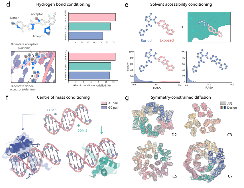
通用任务范围:一个模型覆盖主流“蛋白 + 伙伴”场景
第二个关键点,是它的统一性。RFD3 的设计理念是:用同一组参数,覆盖“几乎所有”常见的“蛋白 + 伙伴分子”相互作用设计场景。不管是对称多聚体、酶催化中心、小分子配体,还是 DNA / RNA 结合,全部都在同一个 all-atom diffusion 框架里处理。
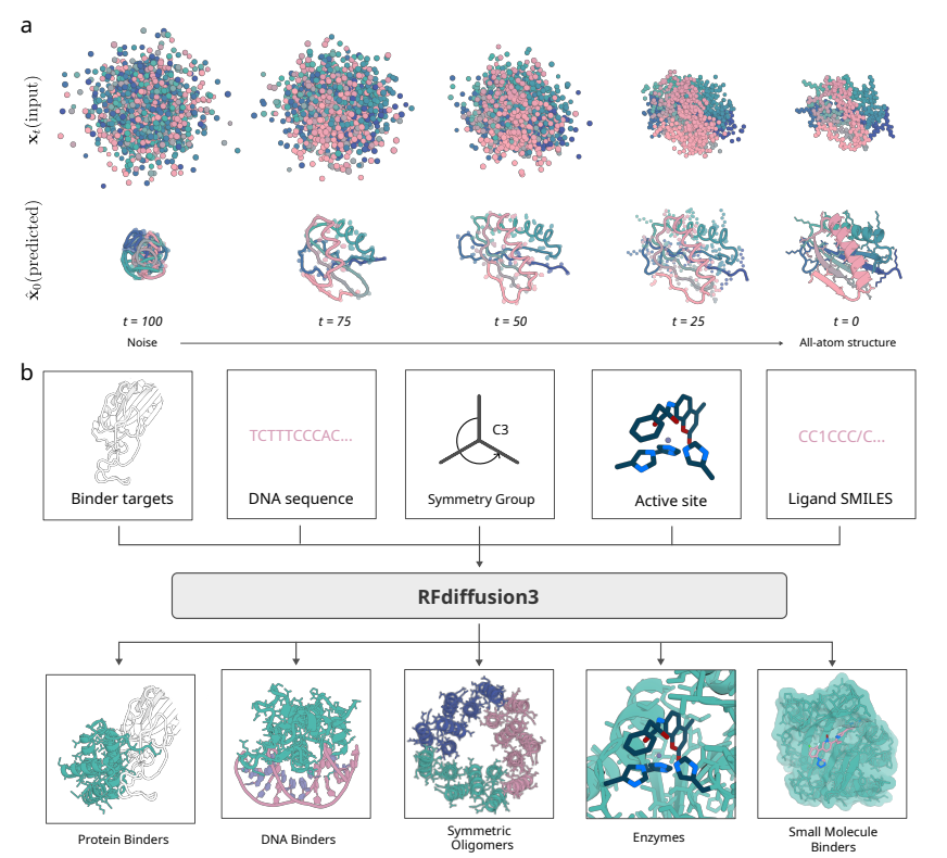
更快也更强:推理效率提升约一个数量级
在 all-atom 分辨率下,反而比前代更快。

设计Binder蛋白与蛋白或核酸结合。
在Binder设计时的参考结构,PDB或CIF格式,可包含蛋白,核酸。
在设计蛋白或核酸的Binder时,从参考结构中选定哪部分作为受体蛋白或核酸。
格式为链名称+残基/碱基编号(UID),多段残基用逗号分隔。例如:参数设置为A25-50,A70-100,A105,A108,/0,B75-108时,表示:
选取参考结构的A链中残基UID为25至50、70至100、105与108的残基/碱基,以及B链UID为75至108的残基/碱基作为受体,同时使用分链符号/0对A与B链之间进行分链,如果不设置分链符,B75的N端会连接在A108的C端。
注意:残基/碱基编号(UID)表示结构文件中带有的编号,该编号可能存在起始编号部位1、间断不连续、或插入编号等情况。当前模型支持插入编号形式,如:A105A表示A链中编号为105A(插入标识为A)的残基。后续所有的残基/碱基编号都是该形式。
定义Binder蛋白的长度,可以是确定的长度,或长度范围,例如:设置为20或20-50时,
20表示Binder蛋白的长度为20个残基;
20-50表示Binder蛋白的长度范围为20至50个残基,具体长度视最终设计结果为准。
指定结构中初始的Binder,从参考蛋白中选定哪部分是初始的Binder蛋白,模型会在不改变初始Binder的前提下,进一步延长Binder,延长的方向通过X指定,例如:参数设置为X,B1-10时,表示:
Length of Binder指定的长度或范围。B1-10,X则表示延长的方向是接在残基B10的C端。选择Receptor Range参数中指定的残基作/碱基为结合位点,格式支持两种形式:
链名称+残基/碱基编号(UID),多段范围用逗号分隔,例如:A59-61,A83,A91,表示:指定A链编号为59至61、83及91的残基/碱基为结合位置。链名称+残基/碱基编号(UID)+原子标准名称,多个原子之间用分号分隔,多段范围用逗号分隔,例如:A83:O;NZ,A91:OG,表示指定A链编号83残基中的O与NZ原子,编号91残基中的OG原子为结合位置。为了方便指定原子,已预定义一批原子组合名称,如下表:| 原子组合名称 | 说明 | 示例 |
|---|---|---|
| ALL | 该残基的所有原子 | A83:ALL表示:指定A链编号83残基中的所有原子 |
| BKBN | 该残基的骨架原子,具体为:N;CA;C;O |
A83:BKBN表示:指定A链编号83残基中的骨架原子 |
| TIP | 残基的主要侧链原子,不同类型残基的TIP原子定义见下方 | A83:TIP表示:指定A链编号83残基中的TIP原子 |
不同类型残基预定义的TIP原子:
"TRP": ["CG","CD1","CD2","NE1","CE2","CE3","CZ2","CZ3","CH2"], # both rings
"HIS": ["CG","ND1","CD2","CE1","NE2"], # ring
"TYR": ["CZ","OH"], # ring dihedral
"PHE": ["CG","CD1","CD2","CE1","CE2","CZ"],
"ASN": ["CB", "CG","OD1","ND2"],
"ASP": ["CB", "CG","OD1","OD2"],
"GLN": ["CG", "CD","OE1","NE2"],
"GLU": ["CG", "CD","OE1","OE2"],
"CYS": ["CB", "SG"],
"SER": ["CB", "OG"],
"THR": ["CB", "OG1"],
"LEU": ["CB", "CG", "CD1", "CD2"],
"VAL": ["CG1", "CG2"],
"ILE": ["CB", "CG2"],
"MET": ["SD", "CE"],
"LYS": ["CE","NZ"],
"ARG": ["CD","NE","CZ","NH1","NH2"],
"PRO": None,
"ALA": None,
"GLY": None,
指定要设计的Binder数量(目前最多支持 100 个)。
包含小分子结构的参考结构,PDB或CIF格式。
参考结构中的小分子名称,如:IAI
注意: 如果小分子名称存在于CCD数据库(https://www.ebi.ac.uk/pdbe-srv/pdbechem/)中时,对应的结构需要一致,否则会报错。如果结构不一致,建议修改小分子名称为L:G或者不在CCD库中的名称,确保名称不重复。
在设计时,从参考结构中提取的小分子中的原子坐标会发生变化,可通过该参数限制某些原子的坐标固定不变。通过结构中的标准原子名称指定,多个原子用逗号分隔,如:N9,O8;C4;C1;N3;C10
指定小分子中的原子,哪些是要掩埋在Binder蛋白的内部(一般是参与相互作用的),不暴露在溶剂中。指定方式同Fixed Ligand Atoms。
指定小分子中的原子,哪些是暴露在溶剂中。指定方式同Fixed Ligand Atoms。
定义Binder蛋白的长度,可以是确定的长度,或长度范围,例如:设置为20或20-50时,
20表示Binder蛋白的长度为20个残基;
20-50表示Binder蛋白的长度范围为20至50个残基,具体长度视最终设计结果为准。
指定要设计的Binder数量(目前最多支持 100 个)。
设计时的酶的参考结构,PDB或CIF格式,可包含酶蛋白与底物分子的全部或部分结构(原子)。
定义酶蛋白的长度,可以是确定的长度,或长度范围,例如:设置为100或100-120
在设计时,从参考结构中提取的结构,固定其中某些原子的坐标不变。原子的指定方式与Binder模式中的Hotspot参数的定位到残基/碱基的原子的方式一致,指定小分子的原子时,使用小分子的名称+原子名称即可,如:IAI:N9;O8
指定从参考结构中提取的结构中,哪些残基的索引由模型推断而非预先指定,残基的选择方式同Binder模式中Receptor Range参数。
指定参考结构中,小分子的名称,提取到设计的复合物结构中,可设置多个,用逗号分隔,如:NAD,IAI
注意: 如果小分子名称存在于CCD数据库(https://www.ebi.ac.uk/pdbe-srv/pdbechem/)中时,对应的结构需要一致,否则会报错。如果结构不一致,建议修改小分子名称为L:G或者不在CCD库中的名称,确保名称不重复。
指定设计的数量,默认为10,最大不超过100
设计时的参考结构,PDB或CIF格式,可包含蛋白,核酸,小分子等。
定义主要的设计策略,指定从参考结构中提取哪部分结构,从头设计哪部分结构等,多段设计策略用逗号分隔。例如:A1-80,10,/0,B5-12,表示:
A1-80的C端,motif的长度也可以指定范围,如24-50,表示设计长度在24至50之间,具体多长看最终的设计结果。指定从参考结构中提取的已知结构,哪部分需要改变序列,多段区域用逗号分隔。例如:‘A20-30,A54-60’,表示Contigs参数中已指定的结构A链残基编号(UID)20至30,54至60的结构部分,需要优化序列。
注意:改变序列的区域一定是在Contigs参数中已指定的,否则会提示错误。
指定整个设计的蛋白的总长度,可以是确定的长度,或长度范围,例如:设置为100或100-200
注意:此处的总长度需大于等于Contigs参数中定义的motif总长度。
指定参考结构中,小分子的名称,提取到设计的复合物结构中,可设置多个,用逗号分隔,如:NAD,IAI
注意: 如果小分子名称存在于CCD数据库(https://www.ebi.ac.uk/pdbe-srv/pdbechem/)中时,对应的结构需要一致,否则会报错。如果结构不一致,建议修改小分子名称为L:G或者不在CCD库中的名称,确保名称不重复。
指定已提取的参考结构中,哪部分是结合位置,格式同Binder模式中的Hotspot参数。
在设计时,从参考结构中提取的残基/碱基或小分子中的原子坐标会发生变化,可通过该参数限制某些原子的坐标固定不变。原子的指定方式与Binder模式中的Hotspot参数的定位到残基/碱基的原子的方式一致,指定小分子的原子时,使用小分子的名称+原子名称即可,如:IAI:N9;O8
指定已提取的参考结构中,哪部分是要掩埋在内部,不暴露在溶剂中。指定方式同Binder模式中的Hotspot参数。可以定位到具体残基/碱基,小分子,也可以精确到具体原子。如指定小分子的某些原子是掩埋的,IAI:N9;O8;C4;C1;N3;C10
指定已提取的参考结构中,哪部分是暴露在溶剂中。指定方式同Buried参数。
指定已提取的参考结构中,哪些原子是作为氢键供体,指定方式同Fixed Atoms参数。
指定已提取的参考结构中,哪些原子是作为氢键受体,指定方式同Fixed Atoms参数。
固定已提取的参考结构的骨架结构不变,只进行侧链的重新设计。
指定生成蛋白的质心(Center of Mass, COM)位置坐标,X,Y,Z坐标通过逗号分隔,如15,2,-4
指定设计的数量,默认为10,最大不超过100
设计得到的结构文件res_design_0_model_0-5.cif
对应的序列文件res_seqs_rfd3.fasta与res_seqs_rfd3_batch.fasta
设计结构的评价Metrics文件metrics_rfd3_summary.csv,包含信息如下:
| 列名 | 说明 |
|---|---|
| Name | 结构名称 |
| max_ca_deviation | 最大CA原子偏差(单位:Å),衡量预测结构与理想结构之间的差异,值越小表示结构越合理,通常应<0.5Å |
| n_chainbreaks | 链断裂数量,表示蛋白主链的连续性,0表示主链完全连续,无断裂 |
| n_clashing.interresidue_clashes_w_sidechain | 残基间侧链冲突数,不同残基侧链间的空间冲突,0表示无侧链冲突 |
| n_clashing.interresidue_clashes_w_backbone | 残基间主链冲突数,不同残基主链间的空间冲突,0表示无主链冲突 |
| non_loop_fraction | 非环区域(螺旋+折叠)占整体结构的比例 |
| loop_fraction | loop区域占整体结构的比例 |
| helix_fraction | alpha螺旋区域占整体结构的比例 |
| sheet_fraction | beta折叠区域占整体结构的比例 |
| num_ss_elements | 二级结构单元数量 |
| radius_of_gyration | 回转半径Rg(单位:Å),衡量蛋白结构的紧密程度,Rg < 15Å:极度紧密的球状结构,通常对应高度稳定的折叠;15-20Å:典型的紧密球蛋白,结构稳定;20-25Å:中等紧密度,可能存在柔性区域;Rg > 25Å:结构较为松散或呈延展构象 |
| alanine_content | 丙氨酸含量,较高的丙氨酸含量有助于螺旋形成 |
| glycine_content | 甘氨酸含量,适中的甘氨酸含量提供结构柔性 |
| num_residues | 总残基数量 |
注意:当前输出结构未进行结构质量的排序,是模型默认的输出顺序。
所有结果的打包文件all_results_rfd3.tar.gz
This module is designed for the de novo design of binder proteins that interact with proteins, nucleic acids, or small molecules. It is based on the RFDiffusion3 (RFD3) model, a diffusion-based protein structure generation framework. RFD3 introduces true multi-molecular co-diffusion, enabling simultaneous modeling of proteins together with their binding partners.
Rather than generating new small-molecule or nucleic-acid sequences from scratch, RFD3 takes chemical entities (e.g., drug-like molecules or nucleic acids) as input and performs diffusion and denoising directly on all atomic coordinates. While generating protein backbone and side-chain atoms, the model simultaneously samples and optimizes the spatial configurations of non-protein molecules, thereby capturing induced-fit effects during binding.
Compared with earlier versions (RFD1/2), RFD3 introduces several major advances:
RFD3 performs diffusion and denoising at the individual atom level, rather than at the residue level. Backbone and side-chain atoms are modeled jointly, allowing geometric and physical constraints to be naturally expressed as conditioning signals, including:
A key strength of RFD3 is its generality. With a single set of model parameters, it supports nearly all common protein + partner design scenarios, including:
All tasks are handled within a unified all-atom diffusion framework.

Despite operating at all-atom resolution, RFD3 is significantly faster than previous versions:
This efficiency allows both finer-resolution modeling and increased sampling within the same GPU time, substantially shortening design iteration cycles.
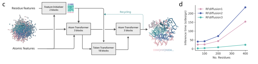
Design binder proteins that interact with proteins, nucleic acids, or small molecules.
The reference structure used for binder design. PDB or CIF format. May contain proteins, nucleic acids, and/or small molecules.
Specifies which parts of the reference structure are treated as the receptor (protein or nucleic acid).
Format: ChainID + Residue/Base UID, with multiple segments separated by commas.
Example:
A25-50,A70-100,A105,A108,/0,B75-108
This selects residues/bases with UID 25–50, 70–100, 105, and 108 from chain A, and UID 75–108 from chain B.
The /0 symbol indicates a chain break between chains A and B. Without it, residue B75 would be connected to the C-terminus of A108.
Note: Residue/base numbering uses the UID as defined in the structure file. This may include non-1 starting indices, gaps, or insertion codes (e.g., A105A). Insertion codes are fully supported.
When designing a small-molecule binder, specify the ligand name from the reference structure.
Defines the length of the binder protein. Can be a fixed length or a range:
20: binder length is exactly 20 residues20-50: binder length ranges from 20 to 50 residuesSpecifies an initial binder fragment extracted from the reference structure. The model extends this fragment without modifying it.
Examples:
X,B1-10: extend from the N-terminus of residue B1B1-10,X: extend from the C-terminus of residue B10Select the residues/nucleotides specified in the Receptor Range parameter as binding sites. Two input formats are supported:
Residue/Nucleotide-level specification
Use chain ID + residue/nucleotide index (UID). Multiple ranges can be separated by commas.
Example: A59-61,A83,A91
This specifies residues/nucleotides with indices 59–61, 83, and 91 on chain A as binding sites.
Atom-level specification within residues/nucleotides
Use chain ID + residue/nucleotide index (UID) + standard atom name. Multiple atoms are separated by semicolons, and multiple ranges are separated by commas.
Example: A83:O;NZ,A91:OG
This specifies atoms O and NZ in residue 83, and atom OG in residue 91 on chain A as binding sites.
Predefined atom groups:
| Atom Group | Description | Example |
|---|---|---|
| ALL | All atoms of the residue | A83:ALL |
| BKBN | Backbone atoms (N;CA;C;O) |
A83:BKBN |
| TIP | Key side-chain atoms (defined per residue type) | A83:TIP |
Predefined TIP atoms by residue type:
"TRP": ["CG","CD1","CD2","NE1","CE2","CE3","CZ2","CZ3","CH2"],
"HIS": ["CG","ND1","CD2","CE1","NE2"],
"TYR": ["CZ","OH"],
"PHE": ["CG","CD1","CD2","CE1","CE2","CZ"],
"ASN": ["CB","CG","OD1","ND2"],
"ASP": ["CB","CG","OD1","OD2"],
"GLN": ["CG","CD","OE1","NE2"],
"GLU": ["CG","CD","OE1","OE2"],
"CYS": ["CB","SG"],
"SER": ["CB","OG"],
"THR": ["CB","OG1"],
"LEU": ["CB","CG","CD1","CD2"],
"VAL": ["CG1","CG2"],
"ILE": ["CB","CG2"],
"MET": ["SD","CE"],
"LYS": ["CE","NZ"],
"ARG": ["CD","NE","CZ","NH1","NH2"],
"PRO": None,
"ALA": None,
"GLY": None
Number of binder designs to generate (maximum: 100).
A reference structure containing the small molecule, in PDB or CIF format.
The name of the small molecule in the reference structure, e.g., IAI.
Note: If the small molecule name exists in the CCD database (https://www.ebi.ac.uk/pdbe-srv/pdbechem/), the corresponding structure must be consistent; otherwise, an error will occur. If the structures are inconsistent, it is recommended to change the small molecule name to L:G or a name not present in the CCD library, ensuring the name is unique.
During design, the coordinates of atoms extracted from the reference structure may change. This parameter allows specific ligand atoms to be fixed so that their coordinates remain unchanged.
Atoms are specified using standard atom names from the structure. Multiple atoms can be separated by commas or semicolons, for example:
N9,O8;C4;C1;N3;C10.
Specifies which ligand atoms should be buried inside the binder protein (typically atoms involved in interactions) and not exposed to the solvent.
The specification format is the same as for Fixed Ligand Atoms.
Specifies which ligand atoms should be exposed to the solvent.
The specification format is the same as for Fixed Ligand Atoms.
Defines the length of the binder protein. This can be a fixed length or a length range, for example 20 or 20-50.
20 means the binder protein has a length of 20 residues.20-50 means the binder protein length ranges from 20 to 50 residues, with the exact length determined by the final design.Specifies the number of binder designs to generate (currently up to a maximum of 100).
The reference structure of the enzyme used during design, in PDB or CIF format. It may include all or part of the enzyme protein and substrate molecules (atoms).
Defines the length of the enzyme. This can be a fixed length or a length range, for example 100 or 100-120.
During design, for structures extracted from the reference structure, the coordinates of specified atoms can be fixed and kept unchanged.
The atom specification format is the same as locating atoms of residues/nucleotides in the Hotspot parameter of the Binder mode.
When specifying atoms of small molecules, use ligand_name + atom_name, for example: IAI:N9;O8.
Specify which residues, among the structures extracted from the reference structure, have their indices inferred by the model rather than being predefined.
The residue selection format is the same as the Receptor Range parameter in the Binder mode.
Specify the names of small molecules in the reference structure to be extracted into the designed complex structure. Multiple ligands can be specified, separated by commas, for example: NAD,IAI.
Note: If the small molecule name exists in the CCD database (https://www.ebi.ac.uk/pdbe-srv/pdbechem/), the corresponding structure must be consistent; otherwise, an error will occur. If the structures are inconsistent, it is recommended to change the small molecule name to L:G or a name not present in the CCD library, ensuring the name is unique.
Specify the number of designs to generate. The default is 10, and the maximum is 100.
The reference structure used during design, in PDB or CIF format. It may include proteins, nucleic acids, small molecules, etc.
Define the main design strategy by specifying which parts are extracted from the reference structure and which parts are designed de novo. Multiple design segments are separated by commas.
For example: A1-80,10,/0,B5-12, which means:
A1-80: First, extract residues 1 to 80 (UID, insertion codes supported) from chain A of the reference structure.10: Design a de novo motif with a length of 10 residues and connect it to the C-terminus of the previous motif A1-80. The motif length can also be specified as a range, such as 24-50, meaning the final length will be determined by the design result./0: A chain break symbol, indicating that the designed protein is split into a new chain at this point, and subsequent motifs belong to a new chain.B5-12: Extract residues 5 to 12 (UID) from chain B of the reference structure.Specify which parts of the extracted known structure need to have their sequences changed. Multiple regions are separated by commas.
For example: A20-30,A54-60 indicates that residues 20–30 and 54–60 (UID) of chain A, which are already specified in the Contigs parameter, need sequence optimization.
Note: The regions to be redesigned must be included in the Contigs parameter; otherwise, an error will be raised.
Specify the total length of the designed protein. This can be a fixed length or a range, for example: 100 or 100-200.
Note: The total length must be greater than or equal to the total motif length defined in the Contigs parameter.
Specify the names of small molecules in the reference structure to be extracted into the designed complex structure. Multiple ligands can be specified, separated by commas, for example: NAD,IAI.
Note: If the small molecule name exists in the CCD database (https://www.ebi.ac.uk/pdbe-srv/pdbechem/), the corresponding structure must be consistent; otherwise, an error will occur. If the structures are inconsistent, it is recommended to change the small molecule name to L:G or a name not present in the CCD library, ensuring the name is unique.
Specify which parts of the extracted reference structure are binding sites. The format is the same as the Hotspot parameter in the Binder mode.
During design, the coordinates of atoms in residues/nucleotides or small molecules extracted from the reference structure may change. This parameter can be used to fix the coordinates of selected atoms so they remain unchanged.
The atom specification format is the same as locating atoms of residues/nucleotides in the Hotspot parameter of the Binder mode.
When specifying atoms of small molecules, use ligand_name + atom_name, for example: IAI:N9;O8.
Specify which parts of the extracted reference structure should be buried inside the protein and not exposed to the solvent.
The specification format is the same as the Hotspot parameter in the Binder mode. It can target specific residues/nucleotides, small molecules, or even specific atoms.
For example, to specify buried atoms of a small molecule: IAI:N9;O8;C4;C1;N3;C10.
Specify which parts of the extracted reference structure should be exposed to the solvent.
The specification format is the same as the Buried parameter.
Specify which atoms in the extracted reference structure act as hydrogen bond donors.
The specification format is the same as the Fixed Atoms parameter.
Specify which atoms in the extracted reference structure act as hydrogen bond acceptors.
The specification format is the same as the Fixed Atoms parameter.
Keep the backbone of the extracted reference structure fixed and redesign only the side chains.
Specify the coordinates of the center of mass (COM) of the generated protein.
The X, Y, and Z coordinates are separated by commas, for example: 15,2,-4.
Specify the number of designs to generate. The default is 10, and the maximum is 100.
res_design_0_model_0-5.cifres_seqs_rfd3.fasta and res_seqs_rfd3_batch.fastametrics_rfd3_summary.csv, which contains the following information:| Column Name | Description |
|---|---|
| Name | Structure name |
| max_ca_deviation | Maximum Cα atom deviation (Å), measuring the difference between the predicted structure and the ideal structure. Smaller values indicate more reasonable structures; typically < 0.5 Å |
| n_chainbreaks | Number of chain breaks, indicating backbone continuity. 0 means the backbone is fully continuous |
| n_clashing.interresidue_clashes_w_sidechain | Number of inter-residue side-chain clashes. 0 indicates no side-chain clashes |
| n_clashing.interresidue_clashes_w_backbone | Number of inter-residue backbone clashes. 0 indicates no backbone clashes |
| non_loop_fraction | Fraction of non-loop regions (helices + sheets) in the overall structure |
| loop_fraction | Fraction of loop regions in the overall structure |
| helix_fraction | Fraction of alpha-helix regions in the overall structure |
| sheet_fraction | Fraction of beta-sheet regions in the overall structure |
| num_ss_elements | Number of secondary structure elements |
| radius_of_gyration | Radius of gyration (Rg, Å), measuring structural compactness. Rg < 15 Å: extremely compact globular structure, typically highly stable; 15–20 Å: typical compact globular protein, stable; 20–25 Å: moderately compact, may contain flexible regions; Rg > 25 Å: relatively loose or extended conformation |
| alanine_content | Alanine content; higher alanine content favors helix formation |
| glycine_content | Glycine content; moderate glycine content provides structural flexibility |
| num_residues | Total number of residues |
Note: The current output structures are not ranked by structural quality; they are presented in the model’s default output order.
all_results_rfd3.tar.gzWeADApt (Wecomput ADA prediction) 是唯信开发的基于多模融合深度学习架构的免疫原性预测系统(也被熟知为AlphaMHC)。
该方法采用全新的多模融合深度神经网络架构,整合了近10亿条与免疫原性相关的湿实验数据(包括亲和力数据、呈递数据、NGS数据、质谱数据等)进行训练,有机地将多个与免疫原性相关的模型融合,构成一个高效的免疫反应模拟系统,可准确地模拟蛋白、抗体、多肽、疫苗等生物药的免疫原性,并能鉴别潜在的免疫原性的T细胞表位(引起临床人体免疫应答的肽段),实现了从序列到临床免疫原性风险的端到端的预测,并通过了数百条来自FDA、EMA的临床真实免疫原性数据(包括单/多特异性抗体和重组蛋白等)的验证测试。

在同样的43个抗体分子的临床ADA数据集上,WeADApt v4.3预测的相关性超过了知名的商业软件EpiMatrix(R2=0.45 vs R2=0.42)。
V4.3版本相对于上个版本v4.2主要有以下改进:
从FDA和EMA的临床试验中收集了200余个已知免疫原性的分子及其ADA的分布,计算模型预测值与真实ADA发生率的相关性,以测试其预测性能。

使用唯信收集整理的200多个临床及上市单抗的ADA数据的测试结果如下图所示,预测分数与ADA发生率的Spearman相关性提升到R=0.74。
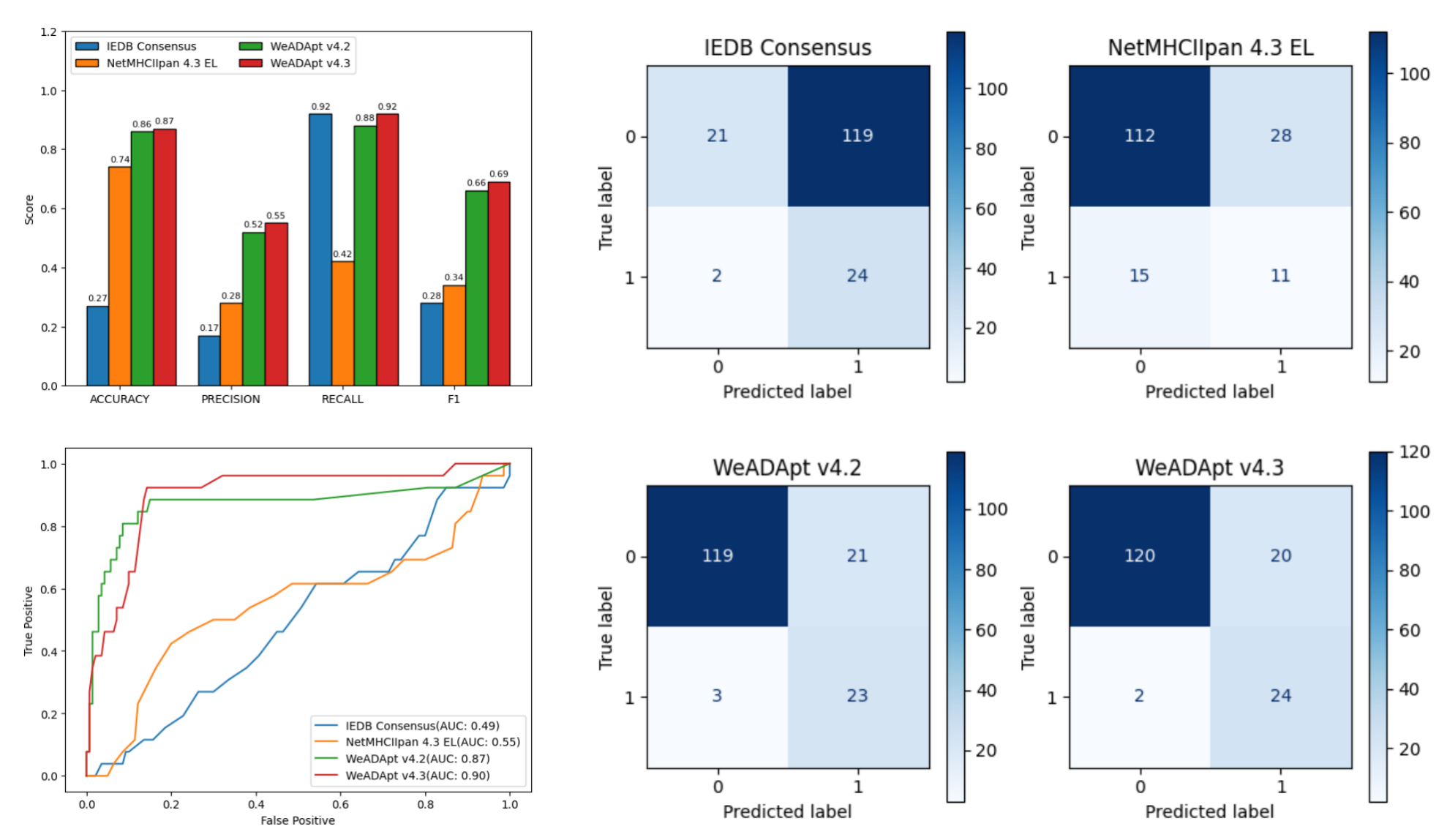
0.2分适合作为单抗的高/低风险的阈值(>20% ADA定义为高风险)。
WeADApt v4被设计为兼容各类的分子形式,不论是对称还是非对称、是否有重复结构域的任意蛋白分子,仅需输入不重复的链即可(重复链全部输入也会自动处理)。
使用唯信收集整理的双抗ADA数据集的测试表现如下图所示,预测分数与ADA发生率的Pearson相关性达到R=0.62。

延续 v4.2 版本的设计,该版本以0.4的分数作为分界线时,可以较好的区分高、低风险的双抗分子。
本系统仅从序列水平预测产生的影响,因此尤其适合同类靶点分子的相对比较和筛选。
待预测的 Fasta 文件。
对序列名有要求,程序内部使用 “蛋白.链名” 的形式区分不同蛋白。
计算量消耗
采用阶梯式动态机制,根据提交的序列数量,对应消耗如下:
蛋白级别的打分和风险评估结果文件。
默认值: MolScore.csv
表位(TCE)明细数据输出文件。
默认值: TceScore.csv
是否导出明细数据。
默认值: no
yes 也不会输出明细是否导出可视化 HTML 报告。
默认值: no
yes 也不会输出报告风险评估阈值。
默认值: 0.2
在表位明细输出中,屏蔽分数 小于该值 的表位。
默认值: 0
蛋白级别的打分和风险评估结果文件MolScore.csv, 表位(TCE)明细数据输出文件TceScore.csv, Details.xlsx文件更详细的数据,用于确认哪些 9 肽对结果影响更大,Plots.tar文件,压缩包中包含可视化报告,每个分子一个独立的 HTML 页面报告。
WeADApt (Wecomput ADA Prediction) is an immunogenicity prediction system developed by Wecomput, based on a multi-modal fusion deep learning architecture. The system is also widely known as AlphaMHC.
This method adopts a novel multi-modal deep neural network framework and is trained on nearly 1 billion experimentally derived immunogenicity-related data points, including binding affinity data, antigen presentation data, NGS data, and mass spectrometry data. By organically integrating multiple immunogenicity-related models, WeADApt constructs an efficient immune response simulation system capable of accurately modeling the immunogenicity of biologics such as proteins, antibodies, peptides, and vaccines.
WeADApt enables end-to-end prediction from sequence to clinical immunogenicity risk, and can identify potential T-cell epitopes that may trigger clinical immune responses. The system has been validated against hundreds of real-world clinical immunogenicity datasets from the FDA and EMA, covering mono-/multi-specific antibodies and recombinant proteins.
On the same clinical ADA dataset comprising 43 antibody molecules, WeADApt v4.3 achieved higher correlation than the well-known commercial software EpiMatrix
(R² = 0.45 vs. R² = 0.42).
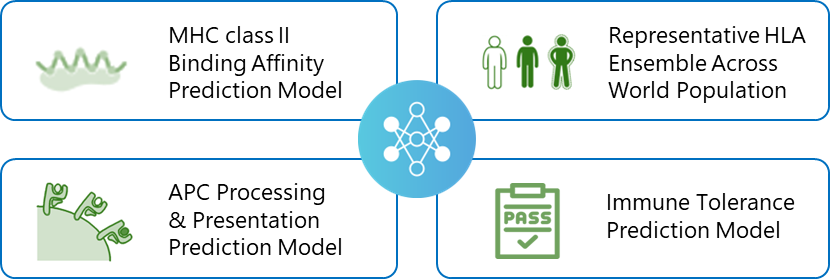
Compared to the previous version (v4.2), V4.3 introduces the following key improvements:
More than 200 molecules with known immunogenicity and corresponding ADA incidence rates were collected from FDA and EMA clinical trials. Model performance was evaluated by measuring the correlation between predicted scores and real ADA incidence rates.

Using a curated dataset of over 200 clinical and marketed monoclonal antibodies, the prediction scores achieved a Spearman correlation of R = 0.74 with observed ADA incidence rates.

A score of 0.2 is recommended as the threshold for distinguishing high- vs. low-risk monoclonal antibodies
(>20% ADA incidence defined as high risk).
WeADApt v4 is designed to be compatible with various molecular formats, including symmetric or asymmetric architectures and proteins with repeated domains. Only non-redundant chains need to be provided as input (duplicate chains are automatically handled by the system).
On a curated bispecific antibody ADA dataset, WeADApt v4 achieved a Pearson correlation of R = 0.62 between predicted scores and observed ADA incidence rates.
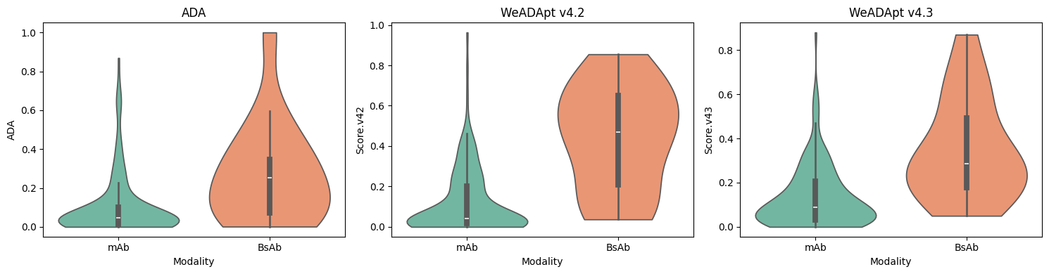
Consistent with v4.2, a score threshold of 0.4 effectively separates high- and low-risk bispecific antibodies in v4.3.
This system predicts immunogenicity solely at the sequence level, making it particularly suitable for relative comparison and screening of molecules targeting the same antigen.
FASTA file containing the sequences to be evaluated.
Sequence identifiers must follow the format “Protein.ChainID”, which is used internally to distinguish different proteins.
WeAdapt 4.3 Pricing Policy
WeAdapt 4.3 uses a tiered, dynamic pricing model, where charges are calculated based on the number of submitted sequences:
Protein-level scoring and immunogenicity risk assessment output file.
Default: MolScore.csv
Output file containing detailed T-cell epitope (TCE) information.
Default: TceScore.csv
Whether to export detailed data.
Default: no
yesWhether to export interactive HTML visualization reports.
Default: no
yesThreshold used for immunogenicity risk assessment.
Default: 0.2
Hide epitopes with scores below this value in the TCE output.
Default: 0
The system generates the following output files:
MolScore.csv: Protein-level scores and immunogenicity risk assessmentTceScore.csv: Detailed T-cell epitope informationDetails.xlsx: Extended data for identifying which 9-mer peptides contribute most significantly to the final scorePlots.tar: Compressed archive containing visualization reports, with one standalone HTML report per molecule将结构A中指定链的C端与结构B中指定链的N端进行拼接,形成新的结构。
用于拼接的结构之一,PDB格式,该结构中指定链的C端参与拼接。
指定结构A中参与拼接的链名,仅单链,如H,如不指定,则默认使用第一条链。
用于拼接的结构之一,PDB格式,该结构中指定链的N端参与拼接。
指定结构B中参与拼接的链名,仅单链,如H,如不指定,则默认使用第一条链。
拼接后的结构名称,默认为join_result.pdb
输出拼接后的结构,默认为join_result.pdb
This module joins two structures by connecting the C-terminus of a specified chain in Structure A with the N-terminus of a specified chain in Structure B, generating a new combined structure.
One of the input structures used for joining, in PDB format.
The C-terminal end of the specified chain in this structure will be used for the join.
The chain in Structure A to be used for joining.
Must be a single chain, e.g., H.
If not specified, the first chain in the structure is used by default.
The second structure used for joining, in PDB format.
The N-terminal end of the specified chain in this structure will be used for the join.
The chain in Structure B to be used for joining.
Must be a single chain, e.g., H.
If not specified, the first chain in the structure is used by default.
Name of the output file containing the joined structure.
Default: join_result.pdb.
The resulting joined structure is written to the output file, with the default name join_result.pdb.
设计能够结合各种生物分子靶标的蛋白、肽类等生物分子。模块基于BoltzGen模型实现,BoltzGen是一个通用的全原子生成模型(all-atom generative model),能够在同一框架下完成多模态的binder设计任务。不同于前代模型只做“推断”,BoltzGen直接在扩散采样过程中生成目标分子与其结合体的全原子结构,并通过可控约束机制确保生成结果物理一致、功能可实现。同时具备良好的泛化性能,能够针对训练过程中未出现过的全新靶标进行有效设计。
BoltzGen的方法设计承接了Boltz系列一贯的目标——在统一的几何表示与能量空间中,学习多模态分子的物理规律。与以往的预测模型不同,BoltzGen 并不输出单一结构预测,而是通过扩散建模(diffusion modeling)直接生成分子的全原子坐标。
其采用扩散模型(diffusion model)框架,在全原子坐标空间中学习分子结构的分布。模型通过在每个采样步骤中向原子坐标加入高斯噪声,再逐步去噪恢复,从而近似真实的势能面分布。与传统的分子生成模型(如仅在残基层面建模)不同,BoltzGen的每个采样变量都是具体原子的位置向量。模型通过能量一致性约束(energy consistency)学习键长、键角、二面角等局部几何关系,从而在生成时自动保持化学合理性。这里对于全原子建模采用了Atom14的方法。
这一设计使生成结构不仅在形状上接近真实蛋白,在能量上也符合分子物理规律。
BoltzGen的架构如下图所示,由三大模块组成:输入层(Input Representation)、条件编码器(Condition Encoder)、扩散模型(Diffusion Model),输出为三维坐标的全原子结构。
BoltzGen的一个突出特点,是并非停留在计算层面的生成验证,而是进行了系统的湿实验评估。进行了十类实验任务(如下图所示),涵盖 蛋白质、肽类、环肽、小分子结合体及抗菌肽设计等多种体系,几乎囊括了现有结构设计模型所能覆盖的全部生物模态。这些实验的共同目标,是检验模型能否在“无同源模板、真实实验条件”下生成可表达、可结合的结构。不同于以往只验证折叠精度的预测模型,BoltzGen的验证标准是功能实现——即所生成分子是否能在实验中稳定结合目标。
BoltzGen 的实验结果显示出较高的一致性与通用性:
在 BoltzGen 论文中,进行抗体和结合蛋白生成的湿实验验证时,抗原(目标蛋白)的主要输入方式是结构,但在特定情况下也可以通过序列输入。
具体说明如下:
默认输入方式:结构
论文中明确提到,除非另有说明,实验中均是将目标的结构(structure)作为输入提供给 BoltzGen 。例如,在针对 9 个新型目标(Novel Targets)设计纳米抗体和蛋白质结合剂时,研究人员利用了目标的结构信息。
灵活性:序列输入与协同折叠(Cofolding) BoltzGen 是一个全原子生成模型,能够同时进行结构预测和蛋白质设计 。当仅提供目标的序列(sequence)作为输入时,模型可以在设计结合剂的同时对目标进行折叠,最终生成结合复合物的原子结构 。
特殊案例:
总结来说,虽然BoltzGen具备直接从序列出发进行设计的能力,但在该论文的大多数湿实验验证(特别是针对新型蛋白目标)中,结构是主要的输入方式。
指定抗体类型,目前支持Antibody(普通抗体)和Nanobody(纳米抗体)。
上传已有的抗原结构,PDB或CIF格式。
指定从结构中提取一些链作为抗原,可多选,如:A,B。如不设置该参数,表示提取结构中的所有链。
指定抗原中的哪些残基参与结合,使用链名+残基位置(从1开始的顺序编号)进行指定,如A10-20,A25,B30-36,B40。
表示:抗原结合位点为A链编号10至20、25的残基,B链提编号30至36、40的残基。
注意:
1.在使用抗原序列文件时,链名是按字母顺序命名(与链的位置顺序对应),第一条链的链名为A,第二条链的链名为B,依次命名。
2.如不设置该参数,模型会自主寻找潜在的结合位点。
支持上传自定义的抗体或纳米抗体模板结构,会采用模板结构的FR区,对CDR区域(Chothia编号)进行重设计,可选择:
.pdb 或 .cif)多个模板结构时,每个模板结构都会用于设计。
如未提供自定义模板,系统将使用内置的默认抗体模板和纳米抗体模板,具体如下:
抗体模板:
6CR1 — Adalimumab(阿达木单抗,Humira)
靶点:TNF-α
作用:阻断 TNF-α 与受体结合,抑制炎症反应
6WGB — Dupilumab(度普利尤单抗,Dupixent)
靶点:IL-4Rα
作用:阻断 IL-4 / IL-13 信号通路,抑制 2 型炎症
3HMW — Ustekinumab(乌司奴单抗,Stelara)
靶点:IL-12 / IL-23 p40
作用:同时抑制 Th1 和 Th17 炎症通路
纳米抗体模板:
7EOW — Caplacizumab(卡普赛珠单抗)
靶点:vWF A1 域
作用:阻断 vWF 与血小板结合,抑制血栓形成
7XL0 — Vobarilizumab(ALX-0061,沃巴利珠单抗)
靶点:IL-6R(+ 白蛋白结合)
作用:抑制 IL-6 信号并延长半衰期
8COH — TPP-3444(Gefurulimab / ALXN1720 组成部分)
靶点:补体 C5
作用:抑制补体激活
8Z8V — ALB8(Ozoralizumab / ATN-103 组件)
靶点:人血清白蛋白(HSA)
作用:延长药物半衰期
Gontivimab(ALX-0171,格替韦单抗)
靶点:RSV F 蛋白
作用:阻断病毒融合,抑制感染
Isecarosmab(M-6495 / ALX-1141,艾司卡索单抗)
靶点:ADAMTS-5
作用:抑制软骨降解,具有抗炎作用
Sonelokimab
靶点:IL-17A / IL-17F
作用:双重抑制炎症因子,增强抗炎效果
完成设计后,最终给出的结构数量,默认为20,最大支持100,设计过程中产生的结构数量在1000左右。
设计模式共有6种:
设计规则的定义有三种方式:
三种方式可以自由组合。
上传已有蛋白结构,从中提取已有结构,或重新设计部分结构。例如:从上传的结构中提取靶点链、抗原链、纳米抗体链等。
指定从Structure中提取的链名,可多选,如:A,B。如不设置该参数,表示提取结构中的所有链。
从Chains参数指定的链中,进一步确认需要提取的残基范围,使用链名+残基位置(从1开始的顺序编号,非PDB的UID编号)进行指定,如A10-20,A25,B1-36,B40。
表示:从A链提取编号10至20、25的残基,从B链提取编号1至36、40的残基。
如不设置该参数,表示提取Chains参数中指定的完整链。
从Chains参数指定的链中,确认哪些残基不提取),与Include参数作用相反,指定方式相同,如A15,B36-42(从1开始的顺序编号,非PDB的UID编号表示A链编号15、B链编号36至42的残基不提取。
已提取的结构中,指定需要重新设计的残基,指定方式同Include参数,如A10-12,B15,B40(从1开始的顺序编号,非PDB的UID编号)。
注意:需要重新设计的残基编号应在已提取的结构中存在。
对要设计的残基,指定二级结构类型。使用链名,SS类型:残基范围(从1开始的顺序编号,非PDB的UID编号)进行指定,每行放置一个,如:
A,HELIX:10-12
B,SHEET:15,LOOP:40
二级结构类型可选:LOOP, HELIX, SHEET(大小写均可)。
不指定该参数表示不强制二级结构类型。
指定哪些残基参与结合(如链间或与小分子结合),指定方式同Include,如A12,B15-18(从1开始的顺序编号,非PDB的UID编号)。
指定哪些残基不参与结合(从1开始的顺序编号,非PDB的UID编号),与Binding参数作用相反。
指定插入突变设计,使用链名,插入位置,插入残基长度,二级结构(从1开始的顺序编号,非PDB的UID编号方式定义,每行一个,如:
A,10,5
B,15,5-10,HELIX
表示在A链的10号残基位置后,插入5个新残基,二级结构不确定(不强制)。在B链的15号残基位置后,插入5至10个残基(具体残基数量随机确定),二级结构为HELIX。
二级结构类型的选择有3种(大小写皆可): LOOP, HELIX, or SHEET
同Structure定义。例如:指定已有的Binder结构。
同Chains定义
同Include定义
同Exclude定义
同Design Positions定义
同Design SS定义
同Binding Hotspot定义
同Non Binding定义
同Design Insertions定义
指定要设计的蛋白序列,每行一条,如:
AAVTTTTPPP
15-20AAAAAAVTTTT18PPP
其中:
18表示序列的该位置将设计18个残基。15-20表示该位置将设计15至20个残基,具体长度在15至20之间随机指定。序列的ID默认从1开始按顺序编号。
指定序列中参与结合的残基,使用序列编号:残基范围格式,如:
1:5,8-10
2:30-35
表示第一条序列中编号5、8至10的残基参与结合;第二条序列中编号30至35的残基参与结合。
第二条序列中含有设计长度范围时,按最小长度计算残基位置。
指定序列中不参与结合的残基,与Sequence_Binding作用相反。
指定序列中残基的二级结构类型,使用序列编号,SS类型:残基范围定义,每行一条,如:
1,HELIX:5-8
2,SHEET:15,LOOP:40
表示第一条序列编号5至8的残基,二级结构为HELIX;第二条序列编号15的残基,二级结构为SHEET,编号40的残基,二级结构为LOOP。
注意: 有指定设计长度范围的序列,按长度最小值来确认剩余残基的位置。
指定需要环化的序列编号,如1,2表示第1和第2条序列首尾相连。
指定参与结合的小分子信息,文本文件,支持SMILES或 CCD Code(化学组分词典编号)。如果使用SMILES格式,每行应包含一个小分子;如果使用CCD Code,每行可以包含一个或多个小分子,使用逗号分隔,并加上CCD前缀。示例如下:
CC(=O)OC1C[NH+]2CCC1CC2
CCD,ATP,HY3,P1L
CCD,MG
共价键信息的文本文件,TXT格式。每行放置一个共价键信息,每个共价键信息包含两个原子信息,每个原子信息由三部分组成:
3,1,CA表示第三个实体(序列或小分子)中的第一个残基(或小分子)的CA原子1,1,CA;2,1,CA1,1,CA,第二个原子为2,1,CA1,1,CA;2,1,CA
1,1,CA;3,1,CHA
当小分子为SMILES时,如CC(=O)NCCNC(C)=O,如果该小分子的顺序编号(按上述方式确认)为3,其第一个C原子参与形成共价键,与编号为1的链/序列中第一个残基的CA原子,则共价键的定义为1,1,CA;3,1,C1其中C1表示小分子的第一个C原子,如果是第二C原子,用C2表示。
注意:
15-20ACS,长度范围的序列长度按最小长度计算,即15,所以残基A的位置编号是16,C是17,S是18。完成设计后,最终给出的结构数量,默认为30,最大支持100,设计过程中产生的结构数量在1000左右。
输出参数文件design_spec.yaml
输出设计的复合物的序列文件,final_complex.fasta
输出设计的复合物的序列文件(Batch模式),final_complex_batch.fasta,适合一些模块的Batch模式的输入,如Structure Prediction (Boltz-2)
输出设计的链的序列文件,final_designed_chains.fasta
输出设计打分文件final_designs_metrics.csv,csv文件每个指标含义如下:
| 列名 | 说明 |
|---|---|
| id | 设计分子的名称 |
| final_rank | 通过各指标综合排序后的最终排名 |
| absolute_score | 基于多种指标(结构指标,物理能量指标)计算的综合打分,但与final rank排序并不完全一致,供参考。 |
| structure_confidence | 基于结构指标(ptm,iptm,pae)计算的结构置信度评分,供参考。 |
| design_ptm | 设计结构的预测TM分数(0–1),反映模型对设计蛋白整体折叠结构的置信度。数值越高表示设计结构越合理,通常 >0.7 视为高置信度。 |
| design_iptm | 设计结构与靶点结构相互作用界面的预测TM分数(0-1),反应相互作用界面质量的置性度。数值越高表示界面结构越合理,通常 >0.7 视为高置信度。 |
| design_to_target_iptm | 仅设计的残基与靶点结构相互作用界面的预测TM分数(0–1),反应相互作用界面质量的置性度。数值越高表示界面结构越合理,通常 >0.7 视为高置信度。 |
| min_design_to_target_pae | 最小预测对齐误差(Å),是残基对水平的置信度指标,用来衡量任意两个残基之间相对空间位置的预测可信度。这里表示设计的结构与靶点结构的残基之间相对位置的准确度。数值越小(例如 <10 Å)准确度越高。 |
| plip_saltbridge_refolded | 重折叠后结构中的盐桥数量。盐桥(带相反电荷残基间的电性作用力)是维持蛋白稳定性的重要因素,数量越多通常结合越稳固。 |
| plip_hbonds_refolded | 重折叠后结构中的氢键数量。氢键是二级结构和界面互补性的关键作用力,数量越多整体稳定性越好。 |
| delta_sasa_refolded | 重折叠前后溶剂可及表面积变化(ΔSASA, Ų)。数值越大(例如 >2000 Ų)表示疏水核心包埋程度越高,通常代表更强的热稳定性。 |
| filter_rmsd | 整个复合物(设计+靶点)结构重折叠后与原设计结构的RMSD值,用于验证生成结构与预测结构的一致性,数值越小越好。 |
| design_ipsae_min | 设计结构与靶点结构之间的最小ipSAE数值(从设计结构出发,计算与靶点结构之间的ipSAE,反之从靶点结构出发,计算与目标结构之间的ipSAE,两者中取最小值)。ipSAE是基于pAE(predicted Aligned Errors)矩阵计算得到的相互作用界面评价分数,取值范围是0到1,值越大,表示预测的蛋白-蛋白相互作用界面越可靠。ipSAE > 0.7 表明相互作用界面预测质量高,结构可信。ipSAE < 0.1: 表明预测中几乎不存在可信互作界面,可排除假阳性相互作用。 |
| design_to_target_ipsae | 从设计结构出发,计算与靶点结构之间的ipSAE。 |
| ALA/GLY/GLU/LEU/VAL/CYS_fraction | 设计的残基中,各类型氨基酸的比例 |
| contacts | 预测结构中的接触界面残基 |
| contacts_overlap | 与输入 hotspot 重叠的预测接触残基 |
| overlap_ratio | 输入 hotspot 被预测接触残基覆盖的比例 |
注意:只有设置Binding Hotspot参数,才会输出contacts、contacts_overlap、overlap_ratio指标
输出设计的前5个结构rank1-5*.cif
输出最后设计的结构打包文件final_designs.tar.gz
输出设计的概述文件results_overview.pdf,包含结构的过滤 (Filtering Criteria)和排序标准(Sorting Criteria)。
| 列名 | 说明 |
|---|---|
| has_x | 阈值:0.0 序列有效性检查。确保序列中不包含未知氨基酸(“X”),必须完全由标准的 20 种天然氨基酸组成,保证序列在物理上可被合成和表达。 |
| filter_rmsd | 阈值:< 2.5 Å 整体骨架的 RMSD。检查整个复合物(设计+靶点)在重折叠后是否保持原样,用于验证生成结构与预测结构的一致性。 |
| filter_rmsd_design | 阈值:< 2.5 Å 仅针对设计部分(Binder)的骨架 RMSD。确保即使靶点有微小移动,结合剂本身的结构依然是稳定的。 |
| designfolding-filter_rmsd | 阈值:< 2.5 Å 独立折叠稳定性检查。在没有靶点的情况下单独折叠结合剂并计算 RMSD。用于确保结合剂能独立折叠,从而大大提高湿实验中的表达成功率。 |
| ALA_fraction GLY_fraction GLU_fraction LEU_fraction VAL_fraction |
阈值:< 0.3 (30%) 序列复杂度/多样性检查。限制丙氨酸、甘氨酸、谷氨酸、亮氨酸、缬氨酸的单项占比。防止模型为了刷高结构稳定性分数而生成单一重复序列,强制要求序列具备化学多样性,以保证特异性的相互作用能力。 |
| 列名 | 说明 |
|---|---|
| design_to_target_iptm | 权重为1 界面预测 TM 得分(0–1),用于评估蛋白–蛋白相互作用界面的结构合理性。数值越大表明界面(如结合位点)越可能形成稳定相互作用。 |
| design_ptm | 权重为1 预测模板建模得分(0–1),反映模型对设计蛋白整体折叠结构的置信度。数值越高表示全局结构越合理,通常 >0.7 视为高置信度。 |
| neg_min_design_to_target_pae | 权重为1 负的最小界面预测对齐误差 (PAE)。PAE 越低越好(误差越小),取负值是为了方便排序(数值越大越好)。它代表模型对结合界面上“最确定的那个接触点”有多大把握。 |
| affinity_probability_binary1 | 权重为1 亲和力预测概率。主要用于小分子结合剂场景。这是模型直接预测出的“该分子能结合”的概率值。 |
| plip_hbonds_refolded | 权重为0.5 重折叠后结构中的氢键数量。氢键是二级结构和界面互补性的关键作用力,数量越多整体稳定性越好。 |
| plip_saltbridge_refolded | 权重为0.5 重折叠后结构中的盐桥数量。盐桥(带相反电荷残基间的电性作用力)是维持蛋白稳定性的重要因素,数量越多通常结合越稳固。 |
| delta_sasa_refolded | 权重为0.5 重折叠前后溶剂可及表面积变化(ΔSASA, Ų)。数值越大(例如 >2000 Ų)表示疏水核心包埋程度越高,通常代表更强的热稳定性。 |
1. 抗体编号
应用WeView打开mH35抗体结构,进行抗体编号,确定重链CDR3的位置在H99-102,为遮蔽肽的结合位置
2. BoltzGen中输入参数设置
1. 抗体编号
应用WeSeq打开mH35抗体序列,进行抗体编号,确定重链CDR3的位置在99-102,为遮蔽肽的结合位置
2. BoltzGen中输入参数设置
The Binder Design module is designed to generate proteins, peptides, and other biomolecules capable of binding to various biological targets. It is implemented based on the BoltzGen model — a universal all-atom generative model capable of performing multimodal binder design tasks within a unified framework. Unlike earlier models that focused solely on “inference,” BoltzGen directly generates the full-atom structures of target molecules and their complexes during diffusion sampling, ensuring physically consistent and functionally feasible results through controllable constraints. It also demonstrates strong generalization, enabling effective design for novel, unseen targets.
The BoltzGen framework inherits the Boltz family’s core objective — to learn the physical laws of multimodal molecules within a unified geometric and energetic representation. Unlike traditional prediction models that output a single structure, BoltzGen uses diffusion modeling to directly generate full atomic coordinates of molecules.
BoltzGen adopts a diffusion model framework to learn molecular structure distributions in full-atom coordinate space. The model adds Gaussian noise to atomic coordinates at each sampling step and progressively denoises them to approximate the real potential energy surface. Unlike traditional residue-level molecular generators, BoltzGen models each atom’s position explicitly. Using energy consistency constraints, the model learns local geometric relationships — such as bond lengths, angles, and torsions — to ensure chemical plausibility during generation. The Atom14 method is used for full-atom representation.
This design ensures that generated structures are not only geometrically realistic but also physically valid in terms of molecular energetics.
The BoltzGen architecture consists of three main modules: Input Representation, Condition Encoder, and Diffusion Model, outputting full-atom 3D coordinates.
A distinguishing feature of BoltzGen is that it goes beyond computational validation and includes extensive wet-lab experimental evaluation. Ten categories of experiments were performed (as shown below), covering proteins, peptides, cyclic peptides, protein–small molecule complexes, and antimicrobial peptides — encompassing nearly all biological modalities addressed by structural design models. The goal was to test whether BoltzGen can generate expressible, functional binders under real experimental conditions without any homologous templates. Unlike models that only validate structural accuracy, BoltzGen emphasizes functional success — i.e., whether the generated molecules can stably bind their targets experimentally.
Experimental results demonstrate high consistency and generality:
In the BoltzGen paper, during wet-lab validation of antibody and binder generation, the primary form of input for the antigen (target protein) is structural information, although sequence-only input is also supported in specific scenarios.
Default Input Mode: Structure
The paper explicitly states that, unless otherwise specified, the target structure is provided as input to BoltzGen in the experiments. For example, when designing nanobodies and protein binders against nine novel targets, the researchers relied on the structural information of the targets.
Flexibility: Sequence Input and Cofolding
BoltzGen is an all-atom generative model capable of performing structure prediction and protein design simultaneously. When only the target sequence is provided, the model can cofold the target and the binder, folding the target while designing the binder and ultimately generating the atomic structure of the bound complex.
Special Cases
No Fixed Structure Input
When designing peptides targeting the disordered region of the NPM1 protein, the researchers adopted a “no fixed structure input” strategy. They provided the structure of the ordered regions of NPM1 while leaving the disordered region flexible, allowing the model to evaluate performance on targets lacking a well-defined structure.
Small-Molecule Targets
For small-molecule targets, BoltzGen requires only a SMILES string (a sequence-based representation of molecular structure) as input and performs cofolding during the design process.
In summary, although BoltzGen is capable of performing design directly from sequence-only inputs, in the majority of the wet-lab validation experiments reported in the paper—especially those involving novel protein targets—structural information was used as the primary form of input.
Specifies the antibody type. Currently supports Antibody (conventional antibodies) and Nanobody.
Upload an existing antigen structure in PDB or CIF format.
Specify which chains in the structure should be extracted as the antigen.
Multiple chains are allowed, e.g., A,B.
If not set, all chains in the structure are used by default.
If no antigen structure is available, you may upload an antigen sequence in FASTA format.
Multi-chain sequences are supported.
Specify which residues on the antigen participate in binding, using the format
ChainName + ResidueIndex (indexing starts from 1), such as:
A10-20,A25,B30-36,B40.
This represents:
Notes:
A, the second is B, and so on.Supports uploading custom antibody or nanobody template structures. The FR regions from the template structures will be adopted, while the CDR regions (Chothia numbering) will be redesigned. Options:
.pdb or .cif)When multiple template structures are provided, each template structure will be used for design.
If no custom template is provided, the system will use built-in default antibody and nanobody templates, listed below:
Antibody Templates
6CR1 — Adalimumab (Humira)
6WGB — Dupilumab (Dupixent)
3HMW — Ustekinumab (Stelara)
Nanobody Templates:
7EOW — Caplacizumab
7XL0 — Vobarilizumab (ALX-0061)
8COH — TPP-3444 (Gefurulimab / ALXN1720 component)
8Z8V — ALB8 (Ozoralizumab / ATN-103 component)
Gontivimab (ALX-0171)
Isecarosmab (M-6495 / ALX-1141)
Sonelokimab
Number of final generated structures. Default: 20, Max: 100. Roughly 1000 candidate structures are sampled during the process.
There are six design modes:
Three approaches to define the design rule:
These approaches can be combined freely.
Upload an existing protein structure to extract or redesign certain regions, e.g., selecting specific chains such as antigen, nanobody, or receptor chains.
Specify chain IDs extracted from Structure, e.g., A,B.
If not set, all chains will be extracted.
From the selected chains (Chains), specify which residues to extract using chainID + residue range, e.g.:
A10-20,A25,B1-36,B40
This extracts residues 10–20 and 25 from chain A, and residues 1–36 and 40 from chain B.
If not set, all residues in Chains are extracted.
Specify residues not to extract from selected chains. Same format as Include, e.g. A15,B36-42.
Specify residues to redesign within the extracted structure, same format as Include, e.g. A10-12,B15,B40.
Note:Must correspond to residues existing in the extracted structure.
Specify secondary structure types for designed residues using the format:
A,HELIX:10-12
B,SHEET:15,LOOP:40
Accepted types: LOOP, HELIX, SHEET (case-insensitive).
If not specified, secondary structures are not constrained.
Define insertion mutations using the format:
A,10,5
B,15,5-10,HELIX
Meaning: insert 5 residues after residue 10 of chain A; insert 5–10 residues after residue 15 of chain B with HELIX conformation.
Accepted secondary structure types: LOOP, HELIX, SHEET.
Specify which residues participate in binding (e.g., between chains or with small molecules), same as Include, e.g. A12,B15-18.
Specify residues not involved in binding.
Same definition as Structure. For example, specify an existing binder structure.
Follow the same rules as the corresponding parameters above.
Follow the same rules as the corresponding parameters above.
Follow the same rules as the corresponding parameters above.
Follow the same rules as the corresponding parameters above.
Follow the same rules as the corresponding parameters above.
Follow the same rules as the corresponding parameters above.
Follow the same rules as the corresponding parameters above.
Follow the same rules as the corresponding parameters above.
Specify the designed protein sequences, one per line, e.g.:
AAVTTTTPPP
15-20AAAAAAVTTTT18PPP
Letters represent fixed residues; numeric values indicate positions to be designed.
Ranges indicate variable lengths (chosen randomly within the range).
Sequence IDs start from 1 by default.
Specify which residues in the sequence are involved in binding:
1:5,8-10
2:30-35
Binding residues are indexed based on the minimum sequence length when ranges are used.
Opposite of Sequence Binding, defines residues not involved in binding.
Define secondary structure for sequence residues:
1,HELIX:5-8
2,SHEET:15,LOOP:40
Positions are determined based on the minimum sequence length when variable ranges exist.
Specify cyclic sequences, e.g. 1,2 means the first and second sequences are cyclized (head-to-tail connected).
Specify small molecules involved in binding.
Supports SMILES or CCD Code formats.
Examples:
CC(=O)OC1C[NH+]2CCC1CC2
CCD,ATP,HY3,P1L
CCD,MG
TXT file defining covalent bonds.
Each line specifies a bond between two atoms using the format:
1,1,CA;2,1,CA
1,1,CA;3,1,CHA
Each atom entry = EntityID,ResidueIndex,AtomName.
Entity IDs are assigned based on the input order of sequences or ligands (starting from 1).
When the small molecule is provided as a SMILES string, e.g. CC(=O)NCCNC(C)=O, if the sequential index of this small molecule (determined as described above) is 3, and its first carbon atom participates in forming a covalent bond with the CA atom of the first residue in chain/sequence 1, then the covalent bond should be defined as:
1,1,CA;3,1,C1
Here, C1 denotes the first carbon atom of the small molecule. If it is the second carbon atom, it should be specified as C2.
Notes:
15-20ACS, the sequence length is taken as 15. Therefore, the position indices are: A = 16, C = 17, S = 18.The covalent bond information is provided as a text file (TXT format).
Each line defines one covalent bond, and each covalent bond consists of two atom definitions.
Each atom definition contains three parts:
Number of final generated structures. Default: 30, Max: 100.
Roughly 1000 candidate structures are sampled during the process.
Output parameter file: design_spec.yaml
Output the sequence file of the designed complex: final_complex.fasta
Output the sequence file of the designed complex (Batch mode): final_complex_batch.fasta, suitable for Batch-mode inputs of some modules, such as Structure Prediction (Boltz-2)
Output the sequence file of the designed chains: final_designed_chains.fasta
Output the design scoring file: final_designs_metrics.csv. The meaning of each metric in the CSV file is as follows:
| Column Name | Description |
|---|---|
| id | Name of the designed molecule |
| final_rank | Final ranking after comprehensive sorting based on all metrics |
| absolute_score | A composite score calculated from multiple metrics (structural metrics and physical energy metrics). It does not fully correspond to the final_rank ordering and is provided for reference. |
| structure_confidence | Structural confidence score calculated from structural metrics (pTM, ipTM, PAE), for reference. |
| design_ptm | Predicted Template Modeling score (0–1), reflecting confidence in the overall fold of the designed protein. Higher values indicate a more reasonable global structure; typically, values >0.7 are considered high confidence. |
| design_to_target_iptm | Interface predicted TM score (0–1), used to evaluate the structural plausibility of the protein–protein interaction interface. Higher values indicate a greater likelihood of forming a stable interface (e.g., binding site). |
| min_design_to_target_pae | Minimum Predicted Alignment Error (Å), a residue-pair–level confidence metric that measures the predicted reliability of relative spatial positions between residues. Here it represents the accuracy of relative positioning between residues of the designed structure and the target structure. Smaller values (e.g., <10 Å) indicate higher accuracy. |
| plip_saltbridge_refolded | Number of salt bridges in the refolded structure. Salt bridges (electrostatic interactions between oppositely charged residues) are important for protein stability; higher numbers generally indicate more stable binding. |
| plip_hbonds_refolded | Number of hydrogen bonds in the refolded structure. Hydrogen bonds are key forces for secondary structure formation and interface complementarity; higher numbers usually imply better overall stability. |
| delta_sasa_refolded | Change in solvent-accessible surface area before and after refolding (ΔSASA, Ų). Larger values (e.g., >2000 Ų) indicate greater burial of the hydrophobic core and usually represent stronger thermal stability. |
| contacts | Contact interface residues in the predicted structure |
| contacts_overlap | Predicted contact residues that overlap with the input hotspots |
| overlap_ratio | Proportion of input hotspots covered by predicted contact residues |
Note: The contacts, contacts_overlap, and overlap_ratio metrics are output only when the Binding Hotspot parameter is set.
Output the top 5 designed structures: rank1-5*.cif
Output the packaged file of the final designed structures: final_designs.tar.gz
The design overview file results_overview.pdf summarizes the Filtering Criteria and Sorting Criteria used for structural evaluation and ranking.
Filtering Criteria
| Column | Description |
|---|---|
| has_x | Threshold: 0.0 Sequence validity check. Ensures that the sequence contains no unknown amino acids (“X”) and is composed exclusively of the 20 standard natural amino acids, guaranteeing physical synthesizability and expressibility. |
| filter_rmsd | Threshold: < 2.5 Å Overall backbone RMSD. Evaluates whether the entire complex (design + target) maintains its structure after refolding, verifying consistency between the generated and predicted structures. |
| filter_rmsd_design | Threshold: < 2.5 Å Backbone RMSD of the designed component (Binder) only. Ensures that the binder itself remains structurally stable even if the target undergoes minor movements. |
| designfolding-filter_rmsd | Threshold: < 2.5 Å Independent folding stability check. The binder is folded without the target, and RMSD is computed to ensure it can fold autonomously, substantially improving the likelihood of successful experimental expression. |
| ALA_fraction GLY_fraction GLU_fraction LEU_fraction VAL_fraction |
Threshold: < 0.3 (30%) Sequence complexity/diversity control. Limits the individual fractions of alanine, glycine, glutamate, leucine, and valine to prevent the model from generating overly repetitive sequences to artificially boost stability scores. This enforces chemical diversity and promotes specific interactions. |
| Column | Description |
|---|---|
| design_to_target_iptm | Weight = 1 Interface Predicted TM score (0–1), used to assess the structural plausibility of the protein–protein interaction interface. Higher values indicate a greater likelihood of forming stable interactions at the interface (e.g., binding sites). |
| design_ptm | Weight = 1 Predicted Template Modeling score (0–1), reflecting confidence in the global fold of the designed protein. Higher values indicate a more plausible overall structure; values >0.7 are typically considered high confidence. |
| neg_min_design_to_target_pae | Weight = 1 Negative minimum Predicted Aligned Error (PAE) at the interface. Lower PAE indicates better accuracy (smaller error); the negative sign is used to facilitate ranking (higher is better). This metric reflects the model’s confidence in the most certain contact point at the binding interface. |
| affinity_probability_binary1 | Weight = 1 Predicted binding affinity probability, primarily used in small-molecule binder scenarios. This is the model’s direct estimate of the probability that the molecule binds. |
| plip_hbonds_refolded | Weight = 0.5 Number of hydrogen bonds in the refolded structure. Hydrogen bonds are critical for secondary structure formation and interface complementarity; higher counts generally indicate better overall stability. |
| plip_saltbridge_refolded | Weight = 0.5 Number of salt bridges in the refolded structure. Salt bridges (electrostatic interactions between oppositely charged residues) are key contributors to protein stability; higher counts typically correspond to stronger binding. |
| delta_sasa_refolded | Weight = 0.5 Change in solvent-accessible surface area upon refolding (ΔSASA, Ų). Larger values (e.g., >2000 Ų) indicate greater burial of hydrophobic cores, generally associated with higher thermal stability. |
1. Antibody Numbering
Open the mH35 antibody structure using WeView, perform antibody numbering, and determine that the heavy chain CDR3 is located at H99-102, which serves as the binding site for the masking peptide
2. Parameter Settings in BoltzGen
1. Antibody Numbering
Open the mH35 antibody sequence using WeSeq, perform antibody numbering, and determine that the heavy chain CDR3 is located at 99-102, which serves as the binding site for the masking peptide
2. Parameter Settings in BoltzGen

基于抗原结构或抗原-抗体复合物结构进行抗体设计,需要有初始抗体序列。模块基于IgGM模型实现。IgGM是一种新型生成式基础模型,旨在加速高亲和力抗体的工程化设计。其学习抗原与抗体之间复杂的结合规律,以及抗体序列与结构之间的映射关系,从而支持多种抗体设计任务。在针对多种抗原的体外实验和计算机模拟基准评估中,其能稳定地产生具有高实测亲和力的抗体或纳米抗体。充分展示了其多样性与高效性,凸显其作为下一代抗体发现与优化强大工具的潜力。
IgGM主要由三个核心组件组成:
IgGM的模型框架如下图所示:
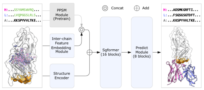
对比结果显示,IgGM在多个CDR区域的预测准确性均高于ProteinMPNN、ProteinMPNN(Filtered)、IgMPNN与IgDesign(如下图所示):
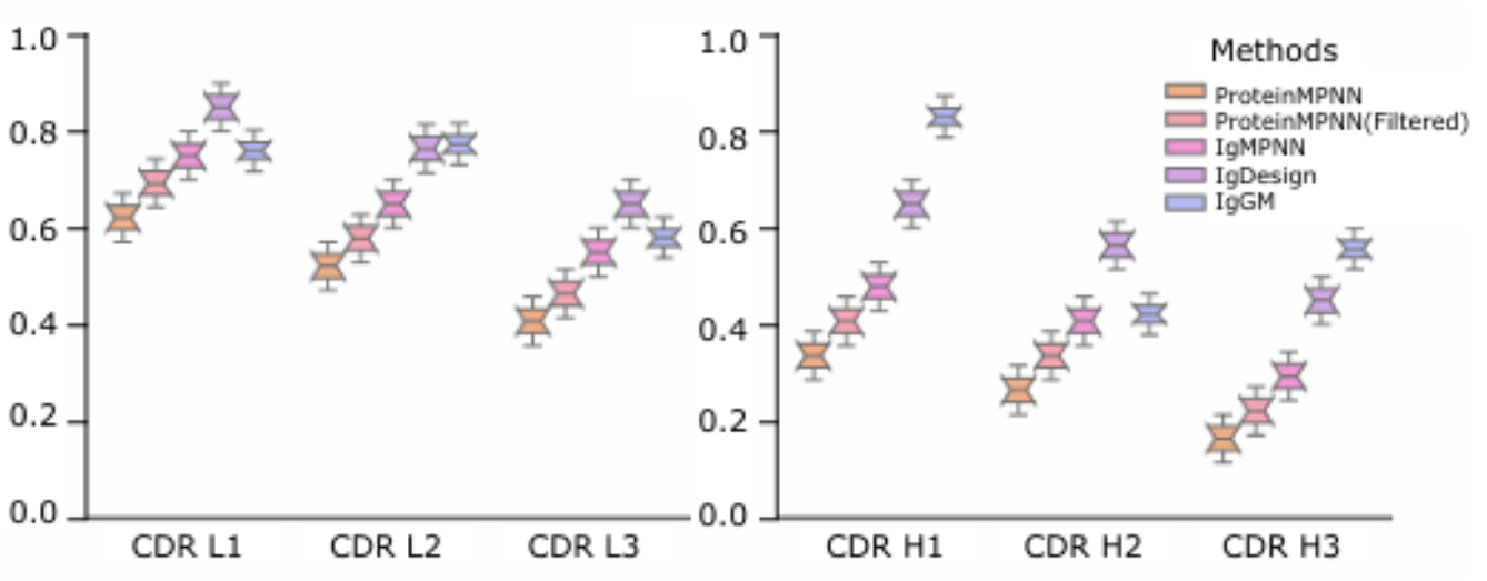
这些结果表明,IgGM的设计与优化策略特别适合捕捉这些关键CDR区域的复杂结构与功能特征,从而提升整体的抗体设计效率。
用于抗体设计的抗体-抗原复合物结构(支持普通抗体或纳米抗体),PDB格式。
注意:当前只支持单链抗原,如存在多链时会默认提取第一条抗原链(或通过后续Chain参数指定抗原链)。
指定抗原链,仅单链。
定义抗体中需要进行设计的残基。
指定格式为:链类型 + 残基编号或编号范围,其中链类型仅支持 H(重链) 和 L(轻链)。
多个残基或编号范围之间使用逗号分隔。
例如,参数设置为:
H27,H28,H99,H100-103,L24-32
表示:
注意:
24-32表示设计所有抗体链中的编号为24-32的残基。指定设计的抗体数量,默认为20,最大支持1000。
指定需要使用的设计模型类型,有三种选择:
指定是否进行结构Relax(使用OpenMM完成),默认不进行。在设计数量较大时,计算时间会显著增加。
指定输出文件的前缀,默认为Result,则输出的文件名称为 Result_编号.fasta 与 Result_编号.pdb
指定抗原的结构文件,PDB格式。当前只支持单链抗原,如存在多链时会默认提取第一条抗原链(或通过后续Chain参数指定抗原链)。
指定抗原链,仅单链。
指定普通抗体Fv区 或者 纳米抗体 的初始序列,fasta格式。如:
>H
QIQLVQSGPELKKPGETVKISCKASGYTFTDYGLNWVKQAPGKGLKWMGWINTYSGEPTYNDEFRGRFAFSLETSTITAYLKINNLKNEDTATYFCARGGNWDWYFDVWGAGTTVTVSS
>L
DIVLTQSPATLSVTPGDNVSLSCRASQIISNNLHWYQQKSHESPRLLIKYASQSISGIPSRFSGSGSGTDFTLSINSVETEDFGMYFCQQSNTWPLTCGSGTKLELN
>nanobody
QVQLVESGGTLVQPGGSLRLSCAASRNISQIAILGWYRQAPGKQREAVAIITGGGPAHYADSVKGRFTISRDTAKNTTYLQMDSLKPEDTAVYFCNVRIRWGAADSWGQGIQVTVSS
定义抗体中需要进行设计的残基。
指定格式为:链类型 + 残基编号或编号范围,其中链类型仅支持 H(重链) 和 L(轻链)。
多个残基或编号范围之间使用逗号分隔。
例如,参数设置为:
H27,H28,H99,H100-103,L24-32
表示:
注意:
24-32表示设计所有抗体链中的编号为24-32的残基。指定抗原链上的结合位点信息,格式:1-5,10,20
同complex模式中的定义。
指定需要使用的设计模型类型,有两种选择:
同complex模式中的定义。
同complex模式中的定义。
seqs.tar.gz。注意:序列排名不分先后。pdbs.tar.gz。:进行分隔。This module performs antibody design based on either antigen structures or antigen–antibody complex structures, requiring an initial antibody sequence as input. The design is powered by the IgGM model, a new generative foundation model developed to accelerate the engineering of high-affinity antibodies. IgGM learns the complex binding relationships between antigens and antibodies, as well as the mapping between antibody sequences and structures, thus enabling various antibody design tasks.
In both in vitro experiments and computational benchmarks across diverse antigens, IgGM consistently generates antibodies and nanobodies with high measured affinity, demonstrating its versatility and efficiency as a next-generation tool for antibody discovery and optimization.
IgGM consists of three core components:
The IgGM model framework is illustrated below:
Comparative results show that IgGM achieves higher prediction accuracy across multiple CDR regions than ProteinMPNN, ProteinMPNN (Filtered), IgMPNN, and IgDesign (see figure below):

These results indicate that IgGM’s design and optimization strategies are particularly well-suited for capturing the complex structural and functional characteristics of critical CDR regions, thereby enhancing the overall efficiency of antibody design.
The antigen–antibody or antigen-nanobody complex structure used for antibody/nanobody design, in PDB format.
Note: Currently, only single-chain antigens are supported. If multiple chains exist, the first chain will be used by default (or the antigen chain can be specified with the Chain parameter).
Specifies the antigen chain (single chain only).
Define the residues in the antibody that need to be redesigned.
The format is Chain Type + Residue Number or Range, where the chain type supports only H (heavy chain) and L (light chain).
Multiple residues or ranges are separated by commas.
For example, if the parameter is set as:
H27,H28,H99,H100-103,L24-32
This means:
Notes:
24-32 designs residues 24–32 in all antibody chains).Specifies the number of antibody designs to generate. Default is 20, maximum is 1000.
Specifies the design model type to use. Three options are available:
Specifies whether to perform structure relaxation using OpenMM. Default is no relaxation.
Note: Relaxation can significantly increase computation time for large design batches.
Specifies the prefix for output files. Default is Result, producing files such as Result_<index>.fasta and Result_<index>.pdb.
Specifies the antigen structure file in PDB format. Only single-chain antigens are supported; for multi-chain structures, the first chain is used by default (or can be specified using Chain).
Specifies the antigen chain (single chain only).
Specifies the initial antibody Fv sequence or nanobody sequence in FASTA format, for example:
>H
QIQLVQSGPELKKPGETVKISCKASGYTFTDYGLNWVKQAPGKGLKWMGWINTYSGEPTYNDEFRGRFAFSLETSTITAYLKINNLKNEDTATYFCARGGNWDWYFDVWGAGTTVTVSS
>L
DIVLTQSPATLSVTPGDNVSLSCRASQIISNNLHWYQQKSHESPRLLIKYASQSISGIPSRFSGSGSGTDFTLSINSVETEDFGMYFCQQSNTWPLTCGSGTKLELN
>nanobody
QVQLVESGGTLVQPGGSLRLSCAASRNISQIAILGWYRQAPGKQREAVAIITGGGPAHYADSVKGRFTISRDTAKNTTYLQMDSLKPEDTAVYFCNVRIRWGAADSWGQGIQVTVSS
Define the residues in the antibody that need to be redesigned.
The format is Chain Type + Residue Number or Range, where the chain type supports only H (heavy chain) and L (light chain).
Multiple residues or ranges are separated by commas.
For example, if the parameter is set as:
H27,H28,H99,H100-103,L24-32
This means:
Notes:
If no chain type is specified, the range applies to all antibody chains (e.g., 24-32 designs residues 24–32 in all antibody chains).
Specifies the binding site information on the antigen chain, in the format: 1-5,10,20.
Same as in the Complex mode.
Specifies the model type, with two options:
Same as in the Complex mode.
Same as in the Complex mode.
seqs.tar.gz.pdbs.tar.gz.:).用于药物发现的高性能ADMET预测平台,帮助研究人员从庞大的化学库和组合化学空间中筛选符合药物性质的小分子。随着高通量分子对接和生成式AI技术的发展,药物化学空间迅速扩大,实验验证的分子选择变得更加重要。ADMET-AI提供快速且准确的吸收、分布、代谢、排泄和毒性预测,实现批量预测。
在性能方面,ADMET-AI在TDC ADMET排行榜上获得了最高的平均排名,同时是目前最快的网页端ADMET预测工具,相较于第二快的公共网页预测服务器,速度提升了45%。在本地运行模式下,对一百万个分子进行预测仅需约3.1小时,极大提高了大规模分子筛选的效率。

小分子SMILES文件,CSV格式。文件内容如下:
smiles,name
O(c1ccc(cc1)CCOC)CC(O)CNC(C)C,lig1
注意
1.小分子SMILES列必须包含列名,示例文件中为smiles。
2.name列用于表示分子名称或标识,可选填写。
CSV文件中小分子SMILES的列名称,例如示例文件中是smiles
预测结果文件,CSV格式。默认为predicted_results.csv。
输出predicted_results.csv文件,包含信息如下:
| 列名 | 含义 |
|---|---|
smiles |
分子的 SMILES 表示法 |
name |
分子名称或标识 |
molecular_weight |
分子量(Da) |
logP |
分子的辛醇/水分配系数,反映疏水性 |
hydrogen_bond_acceptors |
氢键受体数量 |
hydrogen_bond_donors |
氢键供体数量 |
Lipinski |
是否符合 Lipinski 规则(药物可口服性评估) |
QED |
药物化学综合评分(Quantitative Estimate of Drug-likeness) |
stereo_centers |
分子的手性中心数量 |
tpsa |
极性表面积(Topological Polar Surface Area) |
AMES |
AMES 试验预测,评估致突变性 |
BBB_Martins |
跨血脑屏障能力预测(Martins 方法) |
Bioavailability_Ma |
口服生物利用度预测(Ma 方法) |
CYP1A2_Veith |
CYP1A2 酶底物或抑制剂预测(Veith 方法) |
CYP2C19_Veith |
CYP2C19 酶底物或抑制剂预测 |
CYP2C9_Substrate_CarbonMangels |
CYP2C9 底物预测(CarbonMangels 方法) |
CYP2C9_Veith |
CYP2C9 底物/抑制剂预测(Veith 方法) |
CYP2D6_Substrate_CarbonMangels |
CYP2D6 底物预测 |
CYP2D6_Veith |
CYP2D6 底物/抑制剂预测 |
CYP3A4_Substrate_CarbonMangels |
CYP3A4 底物预测 |
CYP3A4_Veith |
CYP3A4 底物/抑制剂预测 |
Carcinogens_Lagunin |
致癌性预测(Lagunin 方法) |
ClinTox |
临床毒性预测 |
DILI |
药物诱导肝损伤(Drug-Induced Liver Injury)预测 |
HIA_Hou |
人体吸收率预测(Hou 方法) |
NR-AR-LBD |
核受体雄激素受体结合域预测 |
NR-AR |
核受体雄激素受体活性预测 |
NR-AhR |
核受体芳烃受体活性预测 |
NR-Aromatase |
芳香酶抑制活性预测 |
NR-ER-LBD |
核受体雌激素受体结合域预测 |
NR-ER |
核受体雌激素受体活性预测 |
NR-PPAR-gamma |
核受体 PPAR-γ 活性预测 |
PAMPA_NCATS |
PAMPA 渗透性预测(NCATS 方法) |
Pgp_Broccatelli |
P-糖蛋白底物预测 |
SR-ARE |
抗氧化反应元件诱导预测 |
SR-ATAD5 |
DNA 损伤修复元件诱导预测 |
SR-HSE |
热休克元件诱导预测 |
SR-MMP |
金属基质蛋白酶诱导预测 |
SR-p53 |
p53 信号通路影响预测 |
Skin_Reaction |
皮肤反应/刺激性预测 |
hERG |
hERG 通道抑制预测(心脏毒性) |
Caco2_Wang |
Caco-2 细胞透过性预测 |
Clearance_Hepatocyte_AZ |
肝细胞清除率预测(AstraZeneca 方法) |
Clearance_Microsome_AZ |
微粒体清除率预测 |
Half_Life_Obach |
半衰期预测(Obach 方法) |
HydrationFreeEnergy_FreeSolv |
水化自由能(FreeSolv 数据库) |
LD50_Zhu |
半数致死量预测(Zhu 方法) |
Lipophilicity_AstraZeneca |
脂溶性预测(AstraZeneca 方法) |
PPBR_AZ |
血浆蛋白结合率(AstraZeneca 方法) |
Solubility_AqSolDB |
水溶性预测(AqSolDB 数据库) |
VDss_Lombardo |
分布容积预测(Lombardo 方法) |
后缀
_drugbank_approved_percentile的列表示对应属性在 DrugBank 批准药物集中的百分位数。例如:
molecular_weight_drugbank_approved_percentile表示该分子分子量在 DrugBank 批准药物中的相对位置(0~100%)。
ADMET-AI is a high-performance ADMET prediction platform for drug discovery, helping researchers screen small molecules with favorable drug-like properties from large chemical libraries and combinatorial chemical spaces. With the development of high-throughput molecular docking and generative AI, the chemical space of potential drugs has rapidly expanded, making the selection of compounds for experimental validation increasingly important. ADMET-AI provides fast and accurate predictions of Absorption, Distribution, Metabolism, Excretion, and Toxicity (ADMET), supporting batch predictions.
In terms of performance, ADMET-AI achieves the highest average rank on the TDC ADMET leaderboard and is currently the fastest web-based ADMET predictor, offering a 45% speed increase compared to the second fastest public web server. In local mode, predictions for one million molecules take only about 3.1 hours, greatly improving the efficiency of large-scale molecular screening.
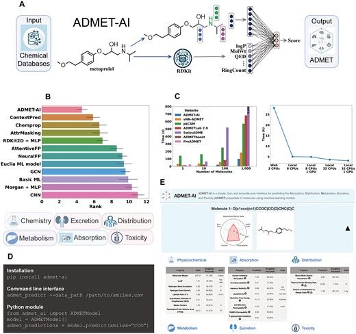
A CSV file containing small molecule SMILES. Example content:
smiles,name
O(c1ccc(cc1)CCOC)CC(O)CNC(C)C,lig1
NOTE:
1.The SMILES column for small molecules must have a header, as shown in the example (smiles).
2.The name column represents the molecule name or identifier and is optional.
The predicted results file in CSV format. Defaults to predicted_results.csv.
The output predicted_results.csv contains the following information:
| Column Name | Meaning |
|---|---|
smiles |
SMILES representation of the molecule |
name |
Molecule name or identifier |
molecular_weight |
Molecular weight (Da) |
logP |
Octanol-water partition coefficient, indicating hydrophobicity |
hydrogen_bond_acceptors |
Number of hydrogen bond acceptors |
hydrogen_bond_donors |
Number of hydrogen bond donors |
Lipinski |
Whether the molecule satisfies Lipinski’s rules (oral drug-likeness) |
QED |
Quantitative Estimate of Drug-likeness (QED) |
stereo_centers |
Number of stereocenters |
tpsa |
Topological Polar Surface Area (TPSA) |
AMES |
AMES mutagenicity prediction |
BBB_Martins |
Blood-brain barrier permeability prediction (Martins method) |
Bioavailability_Ma |
Oral bioavailability prediction (Ma method) |
CYP1A2_Veith |
CYP1A2 substrate/inhibitor prediction (Veith method) |
CYP2C19_Veith |
CYP2C19 substrate/inhibitor prediction |
CYP2C9_Substrate_CarbonMangels |
CYP2C9 substrate prediction (CarbonMangels method) |
CYP2C9_Veith |
CYP2C9 substrate/inhibitor prediction (Veith method) |
CYP2D6_Substrate_CarbonMangels |
CYP2D6 substrate prediction |
CYP2D6_Veith |
CYP2D6 substrate/inhibitor prediction |
CYP3A4_Substrate_CarbonMangels |
CYP3A4 substrate prediction |
CYP3A4_Veith |
CYP3A4 substrate/inhibitor prediction |
Carcinogens_Lagunin |
Carcinogenicity prediction (Lagunin method) |
ClinTox |
Clinical toxicity prediction |
DILI |
Drug-Induced Liver Injury prediction |
HIA_Hou |
Human intestinal absorption prediction (Hou method) |
NR-AR-LBD |
Nuclear receptor androgen receptor ligand binding domain prediction |
NR-AR |
Nuclear receptor androgen receptor activity prediction |
NR-AhR |
Nuclear receptor aryl hydrocarbon receptor activity prediction |
NR-Aromatase |
Aromatase inhibition prediction |
NR-ER-LBD |
Nuclear receptor estrogen receptor ligand binding domain prediction |
NR-ER |
Nuclear receptor estrogen receptor activity prediction |
NR-PPAR-gamma |
Nuclear receptor PPAR-γ activity prediction |
PAMPA_NCATS |
PAMPA permeability prediction (NCATS method) |
Pgp_Broccatelli |
P-glycoprotein substrate prediction |
SR-ARE |
Antioxidant response element induction prediction |
SR-ATAD5 |
DNA damage repair element induction prediction |
SR-HSE |
Heat shock element induction prediction |
SR-MMP |
Matrix metalloproteinase induction prediction |
SR-p53 |
p53 pathway impact prediction |
Skin_Reaction |
Skin reaction / irritation prediction |
hERG |
hERG channel inhibition prediction (cardiotoxicity) |
Caco2_Wang |
Caco-2 cell permeability prediction |
Clearance_Hepatocyte_AZ |
Hepatocyte clearance prediction (AstraZeneca method) |
Clearance_Microsome_AZ |
Microsomal clearance prediction |
Half_Life_Obach |
Half-life prediction (Obach method) |
HydrationFreeEnergy_FreeSolv |
Hydration free energy (FreeSolv database) |
LD50_Zhu |
Lethal dose 50% prediction (Zhu method) |
Lipophilicity_AstraZeneca |
Lipophilicity prediction (AstraZeneca method) |
PPBR_AZ |
Plasma protein binding ratio (AstraZeneca method) |
Solubility_AqSolDB |
Aqueous solubility prediction (AqSolDB database) |
VDss_Lombardo |
Volume of distribution prediction (Lombardo method) |
Columns with the suffix
_drugbank_approved_percentileindicate the percentile of the property relative to approved drugs in DrugBank.
Example:molecular_weight_drugbank_approved_percentileshows the relative position (0–100%) of the molecular weight among approved DrugBank compounds.

批量合并多个CSV文件,并输出合并后的CSV文件。
用于合并的多个CSV文件的打包文件,支持格式:.zip,.tar,.tar.gz,.tgz,.tar.bz2,.tbz2,.tar.xz,.txz
参与合并的单个CSV文件。
参与合并的单个CSV文件。
参与合并的单个CSV文件。
参与合并的单个CSV文件。
参与合并的单个CSV文件。
打包文件或单个CSV文件,可以自由设置,至少设置一个。
指定每个CSV文件需要提取并输出的列,使用文本文件,每行定义一个文件名对应的列名,用英文逗号分隔。未定义的文件,将提取并输出所有列。输出的列名默认是原文件中的列名,如需修改输出的列名称,在对应列名后加上:修改后的列名
示例如下:
ESM_output.csv,Mutation,Log_likelihood,Log_likelihood_target_chain
pythia_output.csv,Mutation,Energy:ddG(pythia)
pythia_ppi_output.csv,Mutation,ddG_Pred:ddG(pythia_ppi)
表示:
ESM_output.csv中提取列Mutation,Log_likelihood,及Log_likelihood_target_chain;pythia_output.csv中提取列Mutation,Energy,同时Energy重命名为pythia(ddG);pythia_ppi_output.csv中提取列Mutation,ddG_Pred,同时ddG_Pred重命名为ddG(pythia_ppi)指定上述提取的列中,用于合并的列名,多列时用逗号分隔,如Mutation表示使用Mutation列进行合并,或者Mutation,Chain表示同时用Mutation,Chain两列进行合并。
注意:如不指定该参数,默认会从各文件的提取列中,选择名称相同的公共列,如没有公共列则无法合并。
过滤方式,目前支持三种方式:TopN,WT,Both:
TopN:对指定的列进行排序,选取排序靠前的N条记录。
WT:对指定的列进行排序,选取数值优于野生型的记录。
Both:同时采用前述两种过滤方式。
指定用于过滤的列名,多列时使用逗号分隔,如:Energy(Pythia),ddG_pred(ThermoMPNN)表示使用列名为Energy(Pythia)及ddG_pred(ThermoMPNN)的列进行过滤。
merged.csv 文件中将新增 Count_Selected 列,用于统计满足筛选条件的列数量。例如,当值为 2 时,表示有两列符合过滤条件。指定Filter Columns参数中,每列的排序方式,1表示升序,0表示降序,与列名顺序对应,通过逗号分隔,如:1,0表示第一个列名用升序,第二个列名用降序。如不设置该参数,则默认都采用升序。
设置TopN过滤方式中的具体N值,正整数。
输出的突变信息和序列中,不包含指定的位点。
格式为:残基位置或范围,如:‘1-10,36’,可加链名,如:‘A1-10,A36’,不加链名时,表示应用到所有可能链的相应位置
进行二次过滤时,对同一位点的所有突变中,仅保留同类型/性质突变残基中的排名最优者,默认为True。
进行二次过滤时,允许同一位点中突变数量的最大值,默认为2,仅保留排名靠前的最大数量突变残基。
用于指定目标链,多条链时使用逗号分隔,如 A,B。在二次筛选阶段,设置后只保留与目标链存在相互作用的突变,不设置则全部保留。如抗原-抗体复合物中,只需保留与抗原链相互作用界面上的突变时,设置该参数为抗原链名,可过滤掉重轻链相互作用界面上的突变。
可加入SASA(relativeSideChain)与Bfactor信息,模块Solvent Exposure (SASA)的输出文件。
是否输出过滤后,相应突变对应的突变序列,单选,Yes或No,默认为Yes。注意:合并后的CSV文件中必须有包含突变信息的列,且突变信息的格式为原残基+突变位置+突变残基(如:G1A),才能进行正常的序列输出。
定义包含突变信息的列名,默认为Mutation。
输出合并文件,默认为merged.csv
输出序列文件的名称,fasta格式,默认为mutated_seqs.fasta
合并输出文件merged.csv。当指定Filter Columns参数时,输出的 merged.csv 文件中将新增:
Hits_Count,用于统计满足筛选条件的列数量。例如,当值为 2 时,表示有两列符合过滤条件。Rank_列名,为该条记录在每个过滤列的排序Rank值。Rank_Avg,满足过滤条件的过滤列的平均Rank值。结果优先按Hits_Count 列降序排序,然后按Rank_Avg列升序排列。
突变序列对应的fasta文件mutated_seqs.fasta,Batch格式的复合物序列文件hits_complex_batch.fasta。
二次过滤后的结果文件,相互作用界面上计算结果
基于合并的计算结果,挑选的相互作用界面上的多样性子集interface_diverse_subset.csv
对相互作用界面上的突变子集,经二次过滤后生成的Batch格式的复合物序列interface_diverse_complex_batch.fasta
对相互作用界面上,经二次过滤后得到的多样性子集,各突变对应的突变序列interface_diverse_mutated_seqs.fasta
对相互作用界面上,经二次过滤后得到的多样性子集,生成双点与三点突变组合,对应的复合物序列。interface_diverse_multi_mutants_complex_batch.fasta
对相互作用界面上,经二次过滤后得到的多样性子集,生成双点与三点突变组合的序列interface_diverse_multi_mutants_seqs.fasta
二次过滤后的结果文件,非相互作用界面上计算结果
non_interface_diverse_subset.csvnon_interface_diverse_complex_batch.fastanon_interface_diverse_mutated_seqs.fastanon_interface_diverse_multi_mutants_complex_batch.fastanon_interface_diverse_multi_mutants_seqs.fasta多链计算结果文件
cross_chain_merged.csv合并后的多链计算结果,包含所有链的综合评分与排序信息。对于多链体系,Cross_Chain_Rank 表示整体综合排名。cross_chain_interface_diverse_subset.csv相互作用界面区域的多样性子集结果。该文件保留界面相关残基/构象中具有代表性的多样化候选,用于分析链间相互作用。cross_chain_non_interface_diverse_subset.csv非相互作用界面区域的多样性子集结果。该文件主要反映非界面区域中的多样化候选分布,用于评估整体结构或序列多样性。Batch merge multiple CSV files and output a single merged CSV file.
A compressed archive containing multiple CSV files to be merged. Supported formats: .zip, .tar, .tar.gz, .tgz, .tar.bz2, .tbz2, .tar.xz, .txz.
A single CSV file to be included in the merge.
A single CSV file to be included in the merge.
A single CSV file to be included in the merge.
A single CSV file to be included in the merge.
A single CSV file to be included in the merge.
Either an archive file or individual CSV files can be provided. At least one must be specified.
Specifies the columns to extract and output from each CSV file. This parameter is provided as a text file, where each line defines the file name and its corresponding column names, separated by commas.
Files not listed will have all columns extracted and output.
By default, output column names are identical to the original names. To rename a column, append :new_name to the original column name.
Example:
ESM_output.csv,Mutation,Log_likelihood,Log_likelihood_target_chain
pythia_output.csv,Mutation,Energy:ddG(pythia)
pythia_ppi_output.csv,Mutation,ddG_Pred:ddG(pythia_ppi)
Meaning:
Mutation, Log_likelihood, and Log_likelihood_target_chain from ESM_output.csv;Mutation and Energy from pythia_output.csv, renaming Energy to ddG(pythia);Mutation and ddG_Pred from pythia_ppi_output.csv, renaming ddG_Pred to ddG(pythia_ppi).Specifies the column names used for merging. Multiple columns should be separated by commas, e.g.,
Mutation (merge by the Mutation column), or
Mutation,Chain (merge using both Mutation and Chain columns).
Note: If this parameter is not specified, the tool will automatically use common columns with identical names among the extracted columns. If no common columns exist, merging cannot be performed.
The filtering method. Three types are supported: TopN, WT, and Both:
Specifies the column names used for filtering. Multiple columns should be separated by commas.
Example:
Energy(Pythia),ddG_pred(ThermoMPNN)
Specifies the sorting order for each column in Filter Columns. 1 indicates ascending order, 0 indicates descending order, correspond to the order of column names, comma-separated; e.g., 1,0 indicates ascending for the first column and descending for the second.
If not specified, all columns default to ascending order.
Defines the N value for the TopN filtering strategy. Must be a positive integer. Default is 20.
The output mutation information and sequences will exclude the specified positions.
The format should be residue indices or ranges, e.g., 1-10,36. Chain identifiers can be included, e.g., A1-10,A36.
If no chain identifier is provided, the positions will be applied to all corresponding residues across all possible chains.
Specifies the column containing mutation information. Default: Mutation.
When performing secondary filtering, whether to retain only interface residues. Default: True.
When performing secondary filtering, for all mutations at the same site, only the top-ranked mutation within each amino acid type/property group is retained. Default: True.
When performing secondary filtering, the maximum number of allowed mutations at the same site. Default: 2. Only the top-ranked mutations up to this maximum are retained.
Specifies the target chain(s). Separate multiple chains with commas, e.g. A,B. During the secondary screening stage, when this parameter is set, only mutations that interact with the target chain(s) are retained; if left unset, all mutations are retained. For example, in an antigen–antibody complex, to retain only mutations on the interaction interface with the antigen chain, set this parameter to the antigen chain name to filter out mutations on the heavy–light chain interaction interface.
Optional inclusion of SASA (relativeSideChain) and B-factor information, using the output file from the Solvent Exposure (SASA) module.
Determines whether to output the mutated sequences corresponding to the filtered variants. Options: Yes or No. Default is Yes.
Note: The merged CSV must contain a column with mutation information in the format
OriginalResidue + Position + MutatedResidue (e.g., G1A) to correctly generate sequences.
Merge the output file into merged.csv. When the Filter Columns parameter is specified, the following columns will be added to the resulting merged.csv:
Hits_Count: counts how many columns meet the filtering criteria. For example, a value of 2 means two columns satisfy the condition.Rank_<ColumnName>: the rank of the record within each filtered column.Rank_Avg: the average rank across all columns that meet the filtering criteria.The results are sorted first by Hits_Count in descending order, then by Rank_Avg in ascending order.
Name of the output FASTA file containing mutated sequences. Default: mutated_seqs.fasta.
The merged output file is merged.csv. When the Filter Columns parameter is specified, the following additional columns will be included in the merged.csv file:
Hits_Count: Counts the number of columns that satisfy the filtering criteria. For example, a value of 2 indicates that two columns meet the filter conditions.Rank_<column_name>: The ranking value of the current record within each filtered column.Rank_Avg: The average rank across all filtered columns that meet the filter conditions.The results are first sorted in descending order by the Hits_Count column, and then in ascending order by the Rank_Avg column.
The FASTA file corresponding to the mutated sequences is mutated_seqs.fasta.
Post-secondary-filtering result files — interaction interface calculation results
interface_diverse_subset.csvinterface_diverse_complex_batch.fastainterface_diverse_mutated_seqs.fastainterface_diverse_multi_mutants_complex_batch.fastainterface_diverse_multi_mutants_seqs.fastaPost-secondary-filtering result files — non-interaction interface calculation results
non_interface_diverse_subset.csvnon_interface_diverse_complex_batch.fastanon_interface_diverse_mutated_seqs.fastanon_interface_diverse_multi_mutants_complex_batch.fastanon_interface_diverse_multi_mutants_seqs.fastaMulti-Chain Result Files
cross_chain_merged.csv: The merged multi-chain calculation results, including the overall scores and ranking information across all chains. In the multi-chain system, Cross_Chain_Rank represents the overall integrated ranking.
cross_chain_interface_diverse_subset.csv: The diversity subset results for interaction interface regions. This file retains representative and diverse candidates among interface-related residues/conformations, and is used to analyze inter-chain interactions.
cross_chain_non_interface_diverse_subset.csv: The diversity subset results for non-interaction interface regions. This file mainly reflects the distribution of diverse candidates in non-interface regions and is used to evaluate overall structural or sequence diversity.
计算蛋白的耐酸性指数,并统计蛋白整体及表面暴露的酸碱性残基及其比例,给出酸性残基集中的区域(Patchs)。
耐酸性指数(ASI)的计算公式为:
ASI = 0.6*碱性残基比例 + 0.3*疏水性残基比例 - 0.5*酸性残基比例
ASI取值范围在-0.5 ~ 0.6之间,越大表示耐酸性能力越强。
表面暴露残基定义为相对溶剂可及表面积(RSA)大于25%的残基。
蛋白结构文件,PDB格式,支持批量,批量格式支持:.zip,.tar,.tar.gz,.tgz,.tar.bz2,.tbz2,.tar.xz,.txz. 目前最大支持1000个结构。
输出蛋白耐酸性指数及各类残基比例等,CSV格式,默认为acid_stability_summary.csv
输出酸性区域残基信息,CSV格式,默认为acid_sensitive_regions.csv
蛋白耐酸性指数及各类残基比例结果文件acid_stability_summary.csv,包含内容如下:
| 列名 | 说明 |
|---|---|
| PDB | 结构文件名称 |
| TotalResidues | 结构中的总残基数量 |
| SurfaceResidues | 表面暴露残基的数量 |
| AcidicRatio | 酸性残基的比例 |
| BasicRatio | 碱性残基的比例 |
| HydrophobicRatio | 疏水残基的比例 |
| SurfaceAcidicRatio | 表面暴露残基中酸性残基的比例 |
| SurfaceBasicRatio | 表面暴露残基中碱性残基的比例 |
| SurfaceHydrophobicRatio | 表面暴露残基中疏水残基的比例 |
| NetCharge@pH2 | 在pH值=2时计算的Net Charge |
| ASI_Global | 基于所有残基计算的耐酸性指数ASI值 |
| ASI_Surface | 仅基于表面暴露残基计算的耐酸性指数ASI值 |
| AcidicPatches | 酸性残基区域的数量 |
酸性区域残基信息文件acid_sensitive_regions.csv
| 列名 | 说明 |
|---|---|
| PDB | 结构文件名称 |
| ClusterID | 酸性残基区域的ID |
| Chain | 所在链名 |
| ResSeq | 组成残基的UID |
| Residue | 残基名 |
Calculates the acid stability index (ASI) of proteins and provides statistics of acidic, basic, and hydrophobic residues in the whole protein and on the surface, along with acidic residue clusters (Patches).
The Acid Stability Index (ASI) is calculated as:
ASI = 0.6*BasicResidueRatio + 0.3*HydrophobicResidueRatio - 0.5*AcidicResidueRatio
ASI ranges from -0.5 ~ 0.6, with higher values indicating stronger acid stability.
Surface-exposed residues are defined as residues with relative solvent accessible surface area (RSA) greater than 25%.
Protein structure files in PDB format. Supports batch processing with formats: .zip, .tar, .tar.gz, .tgz, .tar.bz2, .tbz2, .tar.xz, .txz. The supported maximum number of structures is 1000.
Outputs protein acid stability index and residue ratios in CSV format. Default: acid_stability_summary.csv
Outputs acidic residue cluster information in CSV format. Default: acid_sensitive_regions.csv
The acid stability summary file acid_stability_summary.csv contains:
| Column | Description |
|---|---|
| PDB | Structure file name |
| TotalResidues | Total number of residues in the structure |
| SurfaceResidues | Number of surface-exposed residues |
| AcidicRatio | Ratio of acidic residues |
| BasicRatio | Ratio of basic residues |
| HydrophobicRatio | Ratio of hydrophobic residues |
| SurfaceAcidicRatio | Ratio of acidic residues among surface-exposed residues |
| SurfaceBasicRatio | Ratio of basic residues among surface-exposed residues |
| SurfaceHydrophobicRatio | Ratio of hydrophobic residues among surface-exposed residues |
| NetCharge@pH2 | Net charge calculated at the pH=2 |
| ASI_Global | ASI calculated using all residues |
| ASI_Surface | ASI calculated using only surface-exposed residues |
| AcidicPatches | Number of acidic residue clusters |
The acidic residue cluster file acid_sensitive_regions.csv contains:
| Column | Description |
|---|---|
| PDB | Structure file name |
| ClusterID | ID of the acidic residue cluster |
| Chain | Chain name |
| ResSeq | Residue UID in the cluster |
| Residue | Residue name |
预测抗原中潜在的B细胞表位,及寻找两个抗原之间潜在相似残基。模块基于SEMA模型实现,其中表位预测工具融合了基于序列(SEMA-1D)和基于结构(SEMA-3D)的两种方法:
两个模型均经过微调,用于预测氨基酸残基与免疫球蛋白Fab区的抗原相互作用倾向。此外,表位预测工具还包含一个基于一级序列预测N-糖基化位点的模型,该模型同样基于ESM2。
结合表位预测与相似性比对能够在两个抗原之间识别结构相似的表位,即便抗原整体相似度极低。该功能适用于比较不同病毒或细菌株的蛋白质,其底层神经网络在SaProt模型生成的嵌入向量上训练而成。
用于表位预测的蛋白序列,FASTA格式。最大支持100条序列。
输出评分文件名,CSV格式,默认为result.csv
用于表位预测的蛋白结构,PDB格式。
指定进行表位预测的蛋白链名称,多链用英文逗号分隔,如:A,B。如不指定,表示全部链都进行预测。
输出评分文件名,CSV格式,默认为result.csv
用于N糖基化预测的蛋白序列,FASTA格式。最大支持100条序列。
用于N糖基化预测的蛋白结构,PDB格式。
注意:上述序列和结构,只能选择其一,否则会提示错误
上传结构时,指定进行预测的蛋白链名称,多链用英文逗号分隔,如:A,B。如不指定,表示全部链都进行预测。
输出评分文件名,CSV格式,默认为result.csv
用于比较局部结构相似性的第一个蛋白结构,PDB格式。
指定第一个蛋白用于比较的链名,多链用英文逗号分隔,如:A,B。
指定用于比较局部结构相似性的第二个蛋白结构,PDB格式。
指定第二个蛋白用于比较的链名,多链用英文逗号分隔,如:A,B。
相似残基对的输出文件名,CSV格式,默认为result.csv。相似度值大于2.0时,表示两残基相似,相似度值越大表示残基对越相似。
表位预测的打分文件result.csv,包含如下信息:
| 列名 | 说明 |
|---|---|
| PDB_ID | 结构名称 |
| Chain | 链名称 |
| Residue position | 残基UID编号 |
| AA | 残基单字母名 |
| Epitope_score | 表位预测概率值,表示该残基成为B细胞受体表位的可能性,数值在0-1之间,越大表示成为表位的可能性越高。 |
N糖基化预测的打分文件result.csv,包含如下信息
| 列名 | 说明 |
|---|---|
| PDB_ID | 结构名称 |
| Chain | 链名称 |
| Residue position | 残基UID编号 |
| AA | 残基单字母名 |
| PTM_score | 该残基N是否发生糖基化的概率值,0-1之间,小于0.5表示不会,大于0.5表示会。 |
| PTM_label | 根据PTM_score判断是否会发生N糖基化,0表示不会,1表示会。 |
局部相似性比对结果文件result.csv,包含如下信息:
| 列名 | 说明 |
|---|---|
| PDB_ID_1 | 第一个结构名称 |
| aa_1 | 残基名称 |
| Chain_1 | 链名称 |
| pos_1 | 残基UID编号 |
| PDB_ID_2 | 第二个结构名称 |
| aa_2 | 残基名称 |
| Chain_2 | 链名称 |
| pos_2 | 残基UID编号 |
| score | 相似性打分,数值大于2.0时,表示相似,数值越大相似性越高。 |
Predict potential B-cell epitopes in antigens and identify potentially similar residues between two antigens. This module is implemented based on the SEMA model, which integrates sequence-based (SEMA-1D) and structure-based (SEMA-3D) epitope prediction methods:
Both models are fine-tuned to predict the propensity of amino acid residues to interact with the Fab region of immunoglobulins. Additionally, the epitope prediction tool includes a model for predicting N-glycosylation sites from primary sequences, also based on ESM2. Combining epitope prediction and similarity alignment allows the identification of structurally similar epitopes between two antigens, even when overall antigen similarity is low. This function is suitable for comparing proteins from different viral or bacterial strains, and the underlying neural network is trained on embeddings generated by the SaProt model.
Protein sequence for epitope prediction, in FASTA format. Supports up to 100 sequences.
Output score file name, CSV format, default is result.csv.
Protein structure for epitope prediction, in PDB format.
Specify the protein chains for epitope prediction. Multiple chains are separated by commas, e.g., A,B. If not specified, all chains are predicted.
Output score file name, CSV format, default is result.csv.
Protein sequence for N-glycosylation prediction, FASTA format. Supports up to 100 sequences.
Protein structure for N-glycosylation prediction, PDB format.
Note: Only one of Sequence or Structure can be selected, otherwise an error will occur.
When uploading a structure, specify the chains for prediction. Multiple chains separated by commas, e.g., A,B. If not specified, all chains are predicted.
Output score file name, CSV format, default is result.csv.
The first protein structure for local similarity comparison, PDB format.
Specify chains in the first protein for comparison, multiple chains separated by commas, e.g., A,B.
The second protein structure for local similarity comparison, PDB format.
Specify chains in the second protein for comparison, multiple chains separated by commas, e.g., A,B.
Output file for similar residue pairs, CSV format, default is result.csv. Residue pairs with similarity score greater than 2.0 are considered similar; the higher the score, the more similar the residues.
Epitope prediction score file result.csv contains:
| Column | Description |
|---|---|
| PDB_ID | Structure name |
| Chain | Chain name |
| Residue position | Residue UID |
| AA | Residue single-letter code |
| Epitope_score | Probability of being a B-cell epitope, ranging from 0 to 1; higher values indicate higher likelihood of being an epitope. |
N-glycosylation prediction score file result.csv contains:
| Column | Description |
|---|---|
| PDB_ID | Structure name |
| Chain | Chain name |
| Residue position | Residue UID |
| AA | Residue single-letter code |
| PTM_score | Probability of N-glycosylation at this residue, 0-1; <0.5 indicates unlikely, >0.5 indicates likely. |
| PTM_label | Determined from PTM_score: 0 = not glycosylated, 1 = glycosylated. |
Local similarity comparison result file result.csv contains:
| Column | Description |
|---|---|
| PDB_ID_1 | First structure name |
| aa_1 | Residue name |
| Chain_1 | Chain name |
| pos_1 | Residue UID |
| PDB_ID_2 | Second structure name |
| aa_2 | Residue name |
| Chain_2 | Chain name |
| pos_2 | Residue UID |
| score | Similarity score, >2.0 indicates similar residues; higher values indicate higher similarity. |
生成抗体Fv区序列,或对已有Fv区序列进行序列自然性评分(Log Likelihood)。Fv序列生成支持多种场景:
该功能基于p-IgGen模型实现,p-IgGen是一个专门用于生成抗体重链-轻链配对序列的生成式蛋白质语言模型。由牛津大学与阿斯利康合作开发,其核心目标是生成具有天然抗体特征、且可开发性(developability)良好的抗体序列,用于抗体药物发现。
p-IgGen模型特性如下:
| 特性 | 描述 |
|---|---|
| 训练数据 | 基于 Observed Antibody Space(OAS)数据库,包含约 2.5 亿条非配对序列和 180 万条配对序列 |
| 模型结构 | 自回归解码器(decoder-only),使用旋转位置编码(RoPE),共 1730 万参数 |
| 训练策略 | 阶段训练:非配对预训练(2.5亿条非配对序列,学习抗体序列的语言模式) → 配对微调(180万条配对序列,学习重链与轻链之间的配对关系) |
p-IgGen 的优势:
Generate模式基于已有序列(部分)生成序列
抗体序列,FASTA格式。最大支持500条序列。
generate模式中,表示用于序列生成的部分Fv区序列(模型会在当前序列基础上延展生成新的序列)。
generate模式参数,指定生成的序列数量,默认为10,最大为1000。
generate模式参数,输出生成的序列,FASTA格式。默认为generate.fasta
Pairing Likelihood模式用于抗体重、轻链配对评分
抗体VH(重链Fv区)序列,FASTA格式。最大支持500条序列。
Pairing Likelihood模式中,表示用于序列配对并进行序列评分的VH序列。
抗体VL(轻链Fv区)序列,FASTA格式。最大支持500条序列。
Pairing Likelihood模式中,表示用于序列配对并进行序列评分的VL序列。
输出VH、VL配对后的序列文件,FASTA格式,VH与VL序列通过英文冒号分隔。默认为pairs.fasta
Pairing Likelihood模式参数,输出序列评分文件名,CSV格式,默认为pred_scores.csv
generate模式参数,输入Initial Sequence,输出generate.fastaPairing Likelihood模式参数,输入VH Sequence和VL Sequence,输出pairs.fasta和pred_scores.csv,pred_scores.csv包含以下信息:| 列名 | 说明 |
|---|---|
| Name | 序列名称 |
| Heavy | VH序列名称,进行VH与VL配对评分时输出 |
| Light | VL序列名称,进行VH与VL配对评分时输出 |
| Log Likelihood | 序列自然性评分,数值在 -∞ ~ 0之间,数值越大表示序列越接近天然抗体序列。 |
Generate antibody Fv region sequences or perform naturalness scoring (Log Likelihood) on existing Fv sequences.
Fv sequence generation supports multiple scenarios:
This functionality is powered by the p-IgGen model — a generative protein language model specifically designed for paired antibody heavy-light chain sequence generation.
Developed through collaboration between the University of Oxford and AstraZeneca, p-IgGen aims to generate antibody sequences that exhibit natural antibody-like features and good developability for antibody drug discovery.
| Feature | Description |
|---|---|
| Training Data | Based on the Observed Antibody Space (OAS) database, containing ~250 million unpaired sequences and 1.8 million paired sequences |
| Model Architecture | Decoder-only autoregressive model using Rotary Position Embeddings (RoPE) with 17.3 million parameters |
| Training Strategy | Two-stage training: unpaired pretraining (250M unpaired sequences to learn antibody sequence patterns) → paired fine-tuning (1.8M paired sequences to learn VH–VL pairing relationships) |
High-quality generated sequences
Generated sequences are highly consistent with natural antibodies in terms of sequence similarity, diversity, and CDR length distribution.
They can be successfully modeled by structural modeling tools (e.g., ABodyBuilder2) with high confidence.
Retention of VH/VL pairing information
The model captures natural pairing relationships — generated sequences maintain realistic mutation rates and pairing preferences.
In 94% of tests, real VH/VL pairs scored higher than random pairs.
The Generate mode produces new antibody sequences based on existing (partial) sequences.
Antibody sequences in FASTA format, supporting up to 500 sequences.
In generate mode, this parameter specifies the partial Fv-region sequences on which the model will extend and generate new sequences.
A parameter for generate mode that specifies the number of sequences to generate.
Default: 10; Maximum: 1000.
A parameter for generate mode that specifies the output FASTA file for generated sequences.
Default: generate.fasta.
The Pairing Likelihood mode evaluates the compatibility (pairing likelihood) between antibody heavy- and light-chain sequences.
Antibody VH (heavy-chain Fv region) sequences in FASTA format.
Supports up to 500 sequences.
In Pairing Likelihood mode, this parameter supplies the VH sequences used for chain pairing and likelihood scoring.
Antibody VL (light-chain Fv region) sequences in FASTA format.
Supports up to 500 sequences.
In Pairing Likelihood mode, this parameter supplies the VL sequences used for chain pairing and likelihood scoring.
The FASTA file containing paired VH and VL sequences.
VH and VL sequences are joined using a colon (:).
Default: pairs.fasta.
A Pairing Likelihood mode parameter specifying the CSV file name for likelihood scoring results.
Default: pred_scores.csv.
In Generate mode:
Input: Initial Sequence
Output: generate.fasta
In Pairing Likelihood mode:
Input: VH Sequence and VL Sequence
Output: pairs.fasta and pred_scores.csv
The file pred_scores.csv contains the following fields:
| Column Name | Description |
|---|---|
| Name | Sequence name |
| Heavy | VH sequence name (output when VH–VL pairing is evaluated) |
| Light | VL sequence name (output when VH–VL pairing is evaluated) |
| Log Likelihood | Naturalness score of the sequence. The value ranges from −∞ to 0, and higher values indicate greater similarity to natural antibody sequences. |

设计蛋白高亲和力Binder,可以是线性多肽或小蛋白。模块基于FreeBindCraft实现(FreeBindCraft不同于BindCraft之处在于去掉了商业收费的PyRosetta,使用开源替代),其算法特色在于巧妙利用了AlphaFold2(AF2)的预训练权重,通过反向传播(Backpropagation) 进行“序列幻觉”设计(Hallucination),从头生成能与目标蛋白精准结合的多肽/小蛋白。其自动化流程简洁高效:
与传统方法固定目标蛋白结构不同,FreeBindCraft允许目标和结合剂的骨架均保持一定灵活性,从而能动态“塑形”出完美匹配的界面,更真实地模拟自然界的诱导拟合(Induced Fit)过程。
研究人员在12个极具挑战性的目标上测试了FreeBindCraft,涵盖了细胞受体、过敏原、基因编辑酶等,仅测试少量设计(6-53个)便取得了惊人成果:
实验验证有结合的binder数目及其与Binder长度的分布如下图所示:

有测定亲和力数值的Binder信息如下:
FreeBindCraft不同于BindCraft之处在于去掉了商业收费的PyRosetta,用一套“全开源”组合策略来填补Rosetta 在原流程中的功能空缺,核心思路是:
1.用 GPU 加速的开源物理引擎 OpenMM 替代 Rosetta 的 FastRelax,对复合体做结构松弛,速度提高 2–4 倍;
2.用 MIT 授权的 sc-rs 库计算形状互补(Shape Complementarity),取代 Rosetta InterfaceAnalyzer 的 SC 打分;
3.用 FreeSASA + Biopython 完成表面积/疏水性分析,替换 Rosetta 的界面能量项;
4.结构比对、RMSD 计算等几何操作全部改用 Biopython,彻底去掉 Rosetta 的结构工具依赖;
5.氢键网络评估因预测价值有限,直接舍弃,不再作为强制过滤条件。
实测显示,90%的失败设计在前期已被AlphaFold2筛除,Rosetta能量阈值仅贡献约9%的额外拒绝,因此上述开源替换几乎无损性能。
FreeBindCraft 在速度和效率上显著优于传统 BindCraft,运行快近 3 倍,所需轨迹减少 37%,同时保持设计质量和置信度不变。
| 指标 | 传统 BindCraft (PyRosetta) | FreeBindCraft (开源) | 优势 |
|---|---|---|---|
| 接受设计数 | 101 | 101 | 持平 |
| 所需轨迹数 | 144 | 91 | 减少 37%,更高效 |
| 运行时间 | 33.19 小时 | 12.25 小时 | 快 63%,近 3 倍加速 |
| 平均 ipTM | 0.785 | 0.792 | 持平,略优 |
靶点蛋白的结构,PDB格式。靶点结构中尽量只保留与Binder结合的链,其他链去除,能缩短设计时间。
指定靶点结构中的哪些链作为受体与设计的Binder进行结合,多条链用英文逗号分隔,如:A或者A,B
指定结合位点的残基,支持范围符号,多个区域用英文逗号分隔,如1-10,12,15,如果有多条链时,可以在残基前加上链名来指定,如A1-10,A15,B1-20,B26。
注意:
1.当不指定该参数时,默认使用AF2-multimer预测的结合位点。
2.残基编号为pdb文件的uid
指定需设计的Binder长度,可以是固定长度,或长度范围,如10或者10-30。
注意:
29-40时系统会提示错误。最终设计的Binder数量,默认为10,目前最大支持100,数量越多所需计算时间越长。
不同的Binder长度,设计数量与所需计算时间大致如下:
| Length | Number of Designs | Time(h) |
|---|---|---|
| 65-150 | 100 | ~48 |
| 10 | 10 | ~12 |
| 50 | 10 | ~4 |
| 50 | 100 | ~41 |
| 100 | 10 | ~2 |
| 90-120 | 10 | ~5 |
指定靶点结构是否支持柔性,选中表示靶点链在设计中,其骨架坐标允许1–2Å的RMSD变化,以满足与Binder结合时的诱导契合。
设计的靶点-Binder复合物结构,最多展示前5个。
所有设计结果的打包文件designs.tar.gz
设计结果的详细打分文件final_design_stats.csv
打分指标及其解释见下表:
| 特征 | 描述 |
|---|---|
| MPNN_score | MPNN序列评分,一般不推荐使用,因为依赖于蛋白质本身 |
| MPNN_seq_recovery | MPNN对原始轨迹的序列恢复率 |
| pLDDT | AF2复合物预测的pLDDT置信度评分,归一化到0-1 |
| pTM | AF2复合物预测的pTM置信度评分,归一化到0-1 |
| i_pTM | AF2复合物预测的接口pTM置信度评分,归一化到0-1 |
| pAE | AF2复合物预测的预测对齐误差,归一化(AF2对比n/31)到0-1 |
| i_pAE | AF2复合物预测的接口预测对齐误差,归一化(AF2对比n/31)到0-1 |
| i_pLDDT | AF2复合物预测的接口pLDDT置信度评分,归一化到0-1 |
| ss_pLDDT | AF2复合物预测的二级结构pLDDT置信度评分,归一化到0-1 |
| Unrelaxed_Clashes | 放松前的接口碰撞数量 |
| Relaxed_Clashes | 放松后的接口碰撞数量 |
| Binder_Energy_Score | 单独binder的Rosetta能量评分 |
| Surface_Hydrophobicity | binder表面疏水性分数 |
| ShapeComplementarity | 接口形状互补性 |
| PackStat | 接口PackStat Rosetta得分 |
| dG | 接口Rosetta dG能量 |
| dSASA | 接口delta SASA(面积大小) |
| dG/dSASA | 接口能量除以接口面积 |
| Interface_SASA_% | 接口覆盖binder表面的比例 |
| Interface_Hydrophobicity | binder接口的疏水性比例 |
| n_InterfaceResidues | 接口残基数量 |
| n_InterfaceHbonds | 接口处的氢键数量 |
| InterfaceHbondsPercentage | 氢键数量占接口面积比例 |
| n_InterfaceUnsatHbonds | 接口处未满足的埋藏氢键数量 |
| InterfaceUnsatHbondsPercentage | 未满足埋藏氢键占接口面积比例 |
| Interface_Helix% | 接口处α螺旋比例 |
| Interface_BetaSheet% | 接口处β折叠比例 |
| Interface_Loop% | 接口处环结构比例 |
| Binder_Helix% | binder结构中α螺旋比例 |
| Binder_BetaSheet% | binder结构中β折叠比例 |
| Binder_Loop% | binder结构中环结构比例 |
| InterfaceAAs | 接口处每种氨基酸的数量 |
| HotspotRMSD | binder相对于原始轨迹的未对齐RMSD,即重新预测的复合物中binder与原始结合位点的偏差 |
| Target_RMSD | 在设计的binder背景下预测的目标RMSD,与输入PDB对比 |
| Binder_pLDDT | 单独预测的binder pLDDT置信度评分 |
| Binder_pTM | 单独预测的binder pTM置信度评分 |
| Binder_pAE | 单独预测的binder预测对齐误差 |
| Binder_RMSD | 单独预测的binder RMSD,与原始轨迹对比 |
以N_开头的特征对应每个AlphaFold模型的统计信息,平均值为所有预测模型的平均。
Design high-affinity protein binders, which can be either linear peptides or small proteins.
This module is based on FreeBindCraft (FreeBindCraft differs from BindCraft by removing the commercial PyRosetta dependency, using open-source alternatives instead).
The algorithm leverages AlphaFold2 (AF2) pre-trained weights and performs sequence hallucination via backpropagation, generating de novo peptides/small proteins that bind precisely to target proteins.
The automated workflow is streamlined and efficient:
FreeBindCraft was tested on 12 challenging targets, including cell receptors, allergens, and genome-editing enzymes. Even with only a small number of designs (6–53), it achieved striking results:
Immune checkpoints (PD-1/PD-L1):
Allergen (Bet v1): Designed binders neutralized IgE binding, with a single molecule blocking 50% of IgE–antigen interactions, offering potential for allergy therapy.
Genome editing enzyme (SpCas9): All 6 designs successfully inhibited Cas9 editing activity, providing a precise tool for controlling gene editing.
Viral retargeting (AAV): Mini-binders were designed to redirect adeno-associated virus (AAV) to targets like HER2/PD-L1, boosting gene delivery efficiency up to 100-fold, opening new avenues for gene therapy.
The experimental validation of the number of binders with binding affinity and their distribution relative to Binder length is shown in the figure below:
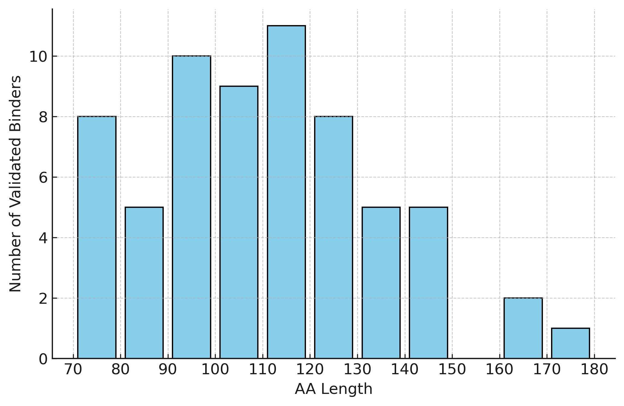
Information on binders with measured affinity values is as follows:
FreeBindCraft replaces Rosetta components with a fully open-source strategy, filling in functional gaps while maintaining performance:
Benchmarks show that ~90% of failed designs were already filtered out by AF2, with Rosetta thresholds only contributing ~9% additional rejection. Thus, these open-source replacements cause negligible performance loss.
FreeBindCraft is almost 3× faster and needs 37 % fewer trajectories while preserving design quality and AlphaFold confidence.
| Metric | BindCraft (PyRosetta) | FreeBindCraft (open source) | Advantage |
|---|---|---|---|
| Accepted designs | 101 | 101 | Equal |
| Trajectories needed | 144 | 91 | –37 %, more efficient |
| Runtime (B200 GPU) | 33.19 h | 12.25 h | –63 %, ≈3× faster |
| Mean ipTM | 0.785 | 0.792 | Equal, slightly better |
The target protein structure, in PDB format. In the target structure, retain only the chain(s) that interact with the Binder and remove all others; this can significantly shorten the design time.
Specify which chains in the target structure are used as receptors for binder design. Multiple chains are separated by commas, e.g. A or A,B.
Specify binding site residues. Range syntax is supported, and multiple ranges are separated by commas, e.g. 1-10,12,15.
For multi-chain targets, prefix residue numbers with chain IDs, e.g. A1-10,A15,B1-20,B26.
Note:
Specify binder length, either as a fixed length or a range, e.g. 10 or 10-30.
Note:
29-40 is invalid and will raise an error.The number of binders to design. Default: 10. Maximum supported: 100.
For different binder lengths, the approximate number of designs and computation time are as follows:
| Length | Number of Designs | Time (h) |
|---|---|---|
| 65–150 | 100 | ~48 |
| 10 | 10 | ~12 |
| 50 | 10 | ~4 |
| 50 | 100 | ~41 |
| 100 | 10 | ~2 |
| 90-120 | 10 | ~5 |
Specify whether the target structure supports flexibility. If selected, target backbones are allowed RMSD changes of 1–2 Å during design to accommodate induced fit.
The designed target–binder complex structures, with the top 5 displayed at most.
All design results are packaged in the file designs.tar.gz.
The detailed scoring file for the design results is final_design_stats.csv.
The features and their explanations are provided in the table below:
| Features | Description |
|---|---|
| MPNN_score | MPNN sequence score, generally not recommended as it depends on protein |
| MPNN_seq_recovery | MPNN sequence recovery of original trajectory |
| pLDDT | pLDDT confidence score of AF2 complex prediction, normalised to 0-1 |
| pTM | pTM confidence score of AF2 complex prediction, normalised to 0-1 |
| i_pTM | interface pTM confidence score of AF2 complex prediction, normalised to 0-1 |
| pAE | predicted alignment error of AF2 complex prediction, normalised compared AF2 by n/31 to 0-1 |
| i_pAE | predicted interface alignment error of AF2 complex prediction, normalised compared AF2 by n/31 to 0-1 |
| i_pLDDT | interface pLDDT confidence score of AF2 complex prediction, normalised to 0-1 |
| ss_pLDDT | secondary structure pLDDT confidence score of AF2 complex prediction, normalised to 0-1 |
| Unrelaxed_Clashes | number of interface clashes before relaxation |
| Relaxed_Clashes | number of interface clashes after relaxation |
| Binder_Energy_Score | Rosetta energy score for binder alone |
| Surface_Hydrophobicity | surface hydrophobicity fraction for binder |
| ShapeComplementarity | interface shape complementarity |
| PackStat | interface packstat rosetta score |
| dG | interface rosetta dG energy |
| dSASA | interface delta SASA (size) |
| dG/dSASA | interface energy divided by interface size |
| Interface_SASA_% | Fraction of binder surface covered by the interface |
| Interface_Hydrophobicity | Interface hydrophobicity fraction of binder interface |
| n_InterfaceResidues | number of interface residues |
| n_InterfaceHbonds | number of hydrogen bonds at the interface |
| InterfaceHbondsPercentage | number of hydrogen bonds compared to interface size |
| n_InterfaceUnsatHbonds | number of unsatisfied buried hydrogen bonds at the interface |
| InterfaceUnsatHbondsPercentage | number of unsatisfied buried hydrogen bonds compared to interface size |
| Interface_Helix% | proportion of alfa helices at the interface |
| Interface_BetaSheet% | proportion of beta sheets at the interface |
| Interface_Loop% | proportion of loops at the interface |
| Binder_Helix% | proportion of alfa helices in the binder structure |
| Binder_BetaSheet% | proportion of beta sheets in the binder structure |
| Binder_Loop% | proportion of loops in the binder structure |
| InterfaceAAs | number of amino acids of each type at the interface |
| HotspotRMSD | unaligned RMSD of binder compared to original trajectory, in other words how far is binder in the repredicted complex from the original binding site |
| Target_RMSD | RMSD of target predicted in context of the designed binder compared to input PDB |
| Binder_pLDDT | pLDDT confidence score of binder predicted alone |
| Binder_pTM | pTM confidence score of binder predicted alone |
| Binder_pAE | predicted alignment error of binder predicted alone |
| Binder_RMSD | RMSD of binder predicted alone compared to original trajectory |
Features starting with N_ correspond to statistics per each AlphaFold model, Averages are accross all models predicted.

SDF File是一个用于指定SDF文件的模块,可用于其他模块的输入。
小分子结构文件,SDF
得到一个与原文件相同的SDF文件
The SDF File module is used to specify an SDF file that can be used as input for other modules.
Small molecule structure file in SDF format.
Obtain an SDF file identical to the original file.
转换包含序列信息的EXCEL或CSV格式文件为序列Fasta格式文件。
Excel或csv格式的文件,必需包含表头信息。
Excel或csv格式文件中,序列ID所在的列名,如:Seq_ID,当该参数未设置时,序列名称默认从1开始进行顺序设置。
Excel或csv格式文件中,序列所在的列名,如:Sequence
设置是否将文件中除去ID与Sequence外的其他列数据,若选择该选项,则将其他列数据以field=value的形式放置在Fasta文件的序列名中。
输出Fasta文件名称,默认为convert.fasta
输出Fasta文件,默认为convert.fasta
Convert sequence information stored in Excel or CSV format files into FASTA format.
Excel or CSV files must include header information.
The column name in the Excel or CSV file that contains the sequence IDs (e.g., Seq_ID).
If this parameter is not specified, sequence IDs will be assigned sequentially starting from 1.
The column name in the Excel or CSV file that contains the sequences (e.g., Sequence).
Set whether to include columns other than ID and Sequence from the file. If this option is selected, the additional columns will be appended to the FASTA sequence name in the format field=value.
The name of the output FASTA file. Default: convert.fasta.
Outputs a FASTA file, with the default name convert.fasta.
Meeko是一个分子预处理工具,主要作用是对输入分子进行标准化和扩展,生成适合后续对接、虚拟筛选或机器学习的分子结构。支持uff, mmff94, mmff94s, espaloma力场
小分子文件,支持Mol (.mol), SD (.sdf), SMILES (.smi )格式,支持单个或批量的小分子输入。
根据指定的pH值(如 --ph 7.4),预测分子的质子化/去质子化状态,并在pH5–9范围内考虑其质子化异构体(protomer)和互变异构体(tautomer)。
默认枚举酸碱异构体,若选择该选项,则跳过酸碱异构体的生成。
默认枚举可能的互变异构体,若选择该选项,则跳过互变异构体的生成。
默认修复六元环的芳香化、张力结构等问题,若选择该选项,则跳过六元环的修复。
默认生成3D构象坐标,若选择该选项,则跳过3D坐标的生成,只保留2D。
3D构象生成相关的参数,用于构象优化的力场,默认为MMFF94。
将分子名称设置为来自SDF文件中小分子属性,如:SDF文件中<IDNUMBER>,可以输入IDNUMBER,作为小分子的名称,适合大批量的小分子输入。
输出文件名称,支持SDF和HDF5格式。
输出结果为优化后的结构文件preprocessed.sdf,每个小分子末尾都会包含ScrubInfo,ScrubInfo包含如下信息:
| 列名 | 说明 |
|---|---|
| isomerGroup | 输入小分子顺序编号(每个分子一个组号) |
| isomerId | 异构体编号信息(同一分子下的不同异构体) |
| confId | 构象编号信息(同一异构体下的不同3D构象) |
| nr_isomers | 该输入分子的异构体总数 |
| nr_conformers | 该输入分子或异构体对应的3D构象总数 |
Meeko is a molecular preprocessing tool that standardizes and expands input molecules, generating structures suitable for subsequent docking, virtual screening, or machine learning. It supports force fields including UFF, MMFF94, MMFF94s, and ESPALOMA.
Input small molecule file, supporting Mol (.mol), SD (.sdf), and SMILES (.smi) formats single or batch small molecule input.
Predicts the protonation/deprotonation states of molecules at a specified pH (e.g., --ph 7.4), considering protomers and tautomers within the pH range of 5–9.
By default, acid-base isomers are enumerated. If this option is selected, acid-base enumeration will be skipped.
By default, possible tautomers are enumerated. If this option is selected, tautomer enumeration will be skipped.
By default, issues in six-membered rings such as aromaticity or ring strain are fixed. If this option is selected, six-membered ring correction will be skipped.
By default, 3D coordinates are generated. If this option is selected, 3D generation is skipped, and only 2D coordinates are retained.
Force field used for conformer optimization. Default is MMFF94.
Set the molecule name from a property in the SDF file, e.g., <IDNUMBER>. You can specify IDNUMBER as the molecule name, which is suitable for batch input of small molecules.
Specifies the output file name. Supports SDF and HDF5 formats.
The output is an optimized structure file preprocessed.sdf. Each molecule includes a ScrubInfo section containing the following information:
| Column Name | Description |
|---|---|
| isomerGroup | Sequential group number of input molecules (one group per molecule) |
| isomerId | Isomer ID (different isomers of the same molecule) |
| confId | Conformer ID (different 3D conformers of the same isomer) |
| nr_isomers | Total number of isomers for the input molecule |
| nr_conformers | Total number of 3D conformers for the input molecule or isomer |
用于从头设计具有理想催化活性的酶。模块基于RFdiffusion2模型,引入流匹配(flow matching)技术替代传统的扩散方法,能够在原子分辨率下直接对酶的活性位点进行骨架化设计,而无需预先指定序列位置或侧链构象,从而显著提高了设计的灵活性与成功率。实验结果表明,RFdiffusion2 不仅在计算基准测试中超越了现有方法,还能生成具备体外催化活性的功能性酶,为从头酶设计开辟了新的可能。

RFdiffusion2在 <100 个酶设计的测试中,就拿到了5种具备实际催化活性的酶;其中一个锌水解酶的活性远超以往工程酶。在Benchmark验证中,从M-CSA数据库中筛选41个真实酶活性位点,每个活性位点提取原子级motif(随机选择催化残基的部分原子)作为输入,使用传统RFdiffusion与RFdiffusion2进行设计,结果显示RFdiffusion2成功解决了41个挑战任务,相比之下,传统的RFdiffusion只能解决其中16个。
在酶设计中,可通过参考结构(如酶活性位点的 Theozyme)作为PDB格式输入。在该结构中引入一个特殊的ORI伪原子(pseudo-atom),用于提供基序放置位置的先验信息。这个伪原子通常放置在酶活性口袋的几何中心,作为目标结构的参考点,引导模型在生成过程中合理定位活性位点及其周围支架的空间关系。
可以使用PyMOL创建该伪原子,方法如下:
# 1️⃣ 选择口袋残基,构建口袋的原子 selection
# 这里假设口袋由 A 链的 11、72、92、94、117、177 号残基组成
select pocket, (resi 11+72+92+94+117+177 and chain A)
# 2️⃣ 在口袋几何中心创建伪原子 ORI
# 参数说明:
# - ORI: 创建的对象名
# - pocket: 使用 selection 的几何中心作为位置
# - name=ORI: 原子名为 ORI
# - resn=ORI: 残基名为 ORI
# - chain=P: 指定链名为 P
# - resi=1: 残基编号为 1
pseudoatom ORI, pocket, name=ORI, resn=ORI, chain=P, resi=1
伪原子格式可以参考:
HETATM 91 ORI ORI B 332 0.000 0.000 0.000 1.00 0.00 X
定义设计策略,可指定多段区域,用英文逗号分隔。例如:该参数设置为 46,A106-106,59,A166-166,2,A169-169,23,A193-193,46,表示:
指定参考结构中,小分子或虚拟原子的名称,可设置多个,用英文逗号分隔,如:NAD,OXM
指定构成活性口袋的原子,通过链名,残基名和原子名称来指定,格式为:链名残基名:原子1名称,原子2名称...,多个残基之间用英文分号分隔。例如:A106:NE,CD,CZ;A166:OD1,CG;A169:NH2,CZ;A193:NE2,CD2,CE1表示:
活性口袋中的原子为:A链残基106中的NE,CD,CZ原子;A链残基166的OD1与CG原子;A链残基169的NH2与CZ原子;A链残基193的NE2,CD2,CE1原子。
指定设计的数量,默认为10,最大不超过100
输出文件的前缀,默认为result,对应的输出文件为result_0.pdb,result_1.pdb…
设计得到的结构文件result_0.pdb,result_1.pdb…
所有结果的打包文件result.tar.gz
注意:
A tool for de novo design of enzymes with desired catalytic activity. The module is based on the RFdiffusion2 model, which introduces flow matching to replace traditional diffusion methods. It enables atom-level scaffold design of enzyme active sites directly, without predefining sequence positions or side-chain conformations, thus significantly improving design flexibility and success rates. Experimental results show that RFdiffusion2 not only outperforms existing methods in computational benchmarks but also generates functional enzymes with in vitro catalytic activity, opening new possibilities for de novo enzyme design.
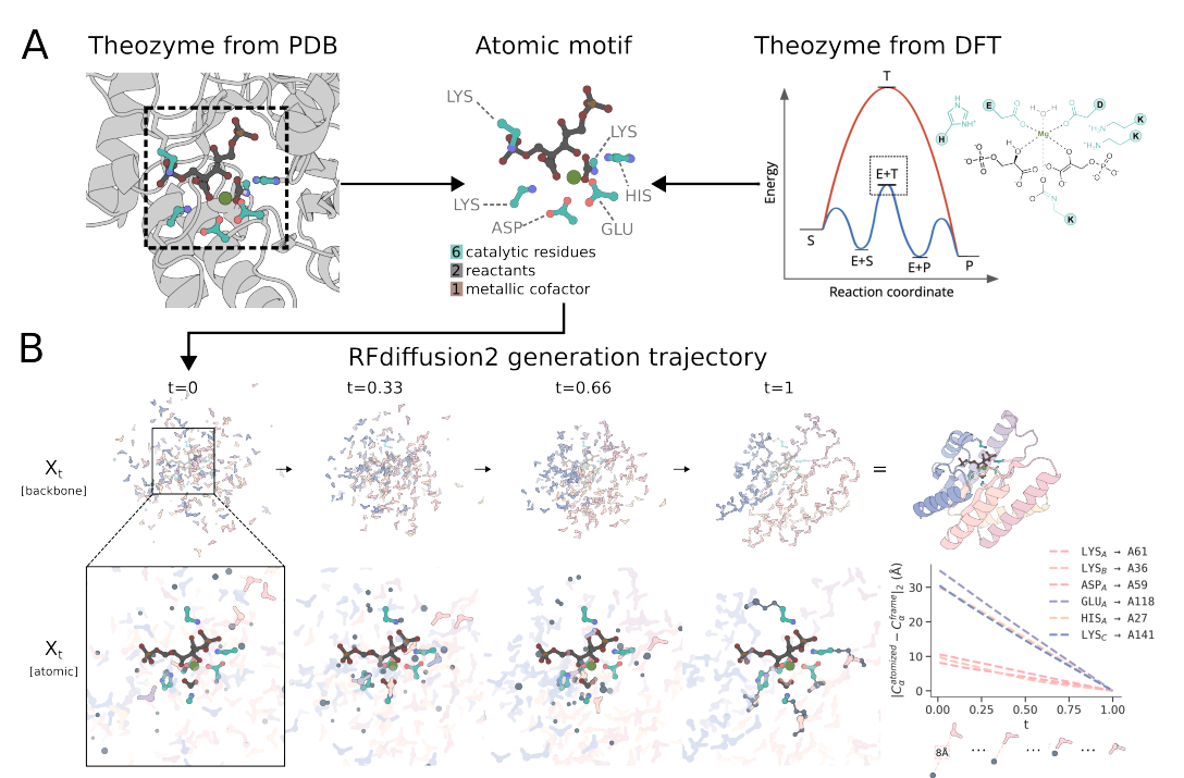
In a test of fewer than 100 designed enzymes, RFdiffusion2 successfully produced 5 enzymes with actual catalytic activity; among them, one zinc hydrolase exhibited activity far surpassing previous engineered enzymes. In benchmark validation, 41 real enzyme active sites were extracted from the M-CSA database. For each site, atomic-level motifs (randomly selecting atoms from catalytic residues) were used as inputs for design by both traditional RFdiffusion and RFdiffusion2. The results showed that RFdiffusion2 successfully solved all 41 challenge cases, whereas traditional RFdiffusion solved only 16.
In enzyme design, a reference structure (such as the Theozyme of the enzyme active site) can be provided in PDB format.
Within this structure, a special ORI pseudo-atom is introduced to provide prior spatial information for motif placement.
This pseudo-atom is typically positioned at the geometric center of the enzyme active pocket, serving as a reference point to guide the model in properly aligning the active site with the surrounding scaffold during the design process.
The pseudo-atom can be created in PyMOL as follows:
# 1️⃣ Select the residues that form the binding pocket
# Example: pocket consists of residues 11, 72, 92, 94, 117, 177 in chain A
select pocket, (resi 11+72+92+94+117+177 and chain A)
# 2️⃣ Create a pseudo-atom (ORI) at the geometric center of the pocket
# Parameter explanation:
# - ORI: name of the created object
# - pocket: use the geometric center of this selection as position
# - name=ORI: atom name set to ORI
# - resn=ORI: residue name set to ORI
# - chain=P: assign chain identifier as P
# - resi=1: assign residue number as 1
pseudoatom ORI, pocket, name=ORI, resn=ORI, chain=P, resi=1
The pseudo-atom in the exported PDB file will follow a format similar to:
HETATM 91 ORI ORI B 332 0.000 0.000 0.000 1.00 0.00 X
Defines the design strategy. Multiple segments can be specified, separated by commas.
Example:
46,A106-106,59,A166-166,2,A169-169,23,A193-193,46
This means:
46: first design a motif of length 46 (a range can also be specified, e.g., 24-50, meaning a random length between 24 and 50).A106-106: then take residue 106 from chain A of the reference protein, attaching its N-terminus to the C-terminus of the previously designed 46-length motif (a range such as A100-118 can also be given to take residues 100–118 from chain A).59: design a motif of length 59, attached to the previous motif’s C-terminus.A166-166: take residue 166 from chain A, attach its N-terminus to the previous motif’s C-terminus.2: design a motif of length 2, attached to the previous motif’s C-terminus.A169-169: take residue 169 from chain A, attach to the previous motif’s C-terminus.23: design a motif of length 23, attached to the previous motif’s C-terminus.A193-193: take residue 193 from chain A, attach to the previous motif’s C-terminus.46: design another motif of length 46, attached to the previous motif’s C-terminus.Specifies small molecules or dummy atoms in the reference structure. Multiple ligands can be listed, separated by commas, e.g., NAD,OXM.
Defines the atoms that make up the active pocket. Specified by chain ID, residue number, and atom names.
Format:
ChainResidue:Atom1,Atom2...
Multiple residues are separated by semicolons.
Example:
A106:NE,CD,CZ;A166:OD1,CG;A169:NH2,CZ;A193:NE2,CD2,CE1
This means:
Specify the number of designs; the default is 10, and the maximum allowed is 100.
Prefix for the output files; the default is result, yielding files named result_0.pdb, result_1.pdb, …
Structure files generated by the design: result_0.pdb, result_1.pdb, …
An archive containing all results: result.tar.gz
Notes:

GenMol是基于diffusion model的开源AI框架,用于分子生成。它从大型化学数据库中学习,生成类药物分子。GenMol能够同时优化多种属性(类药物特性、合成可得性),并提供合成规划,大致确保分子可在实验室中合成。
GenMol支持多种生成模式,满足不同的药物发现需求:
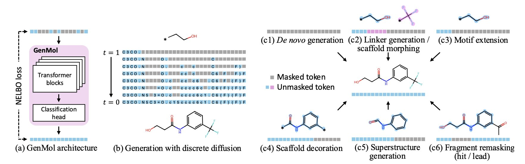
选择生成模式:Superstructure-Generation、Scaffold-Decoration、Motif-Extension、Linker-Design
分子结构文件,格式为SDF或SMILES,文件后缀为.sdf/.sd或.smi
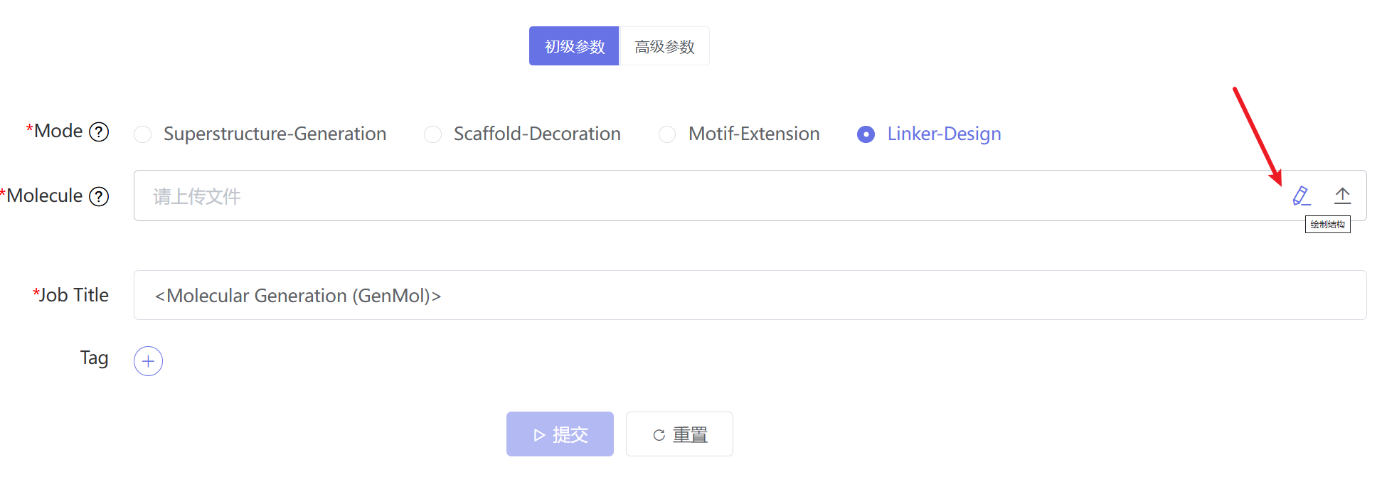
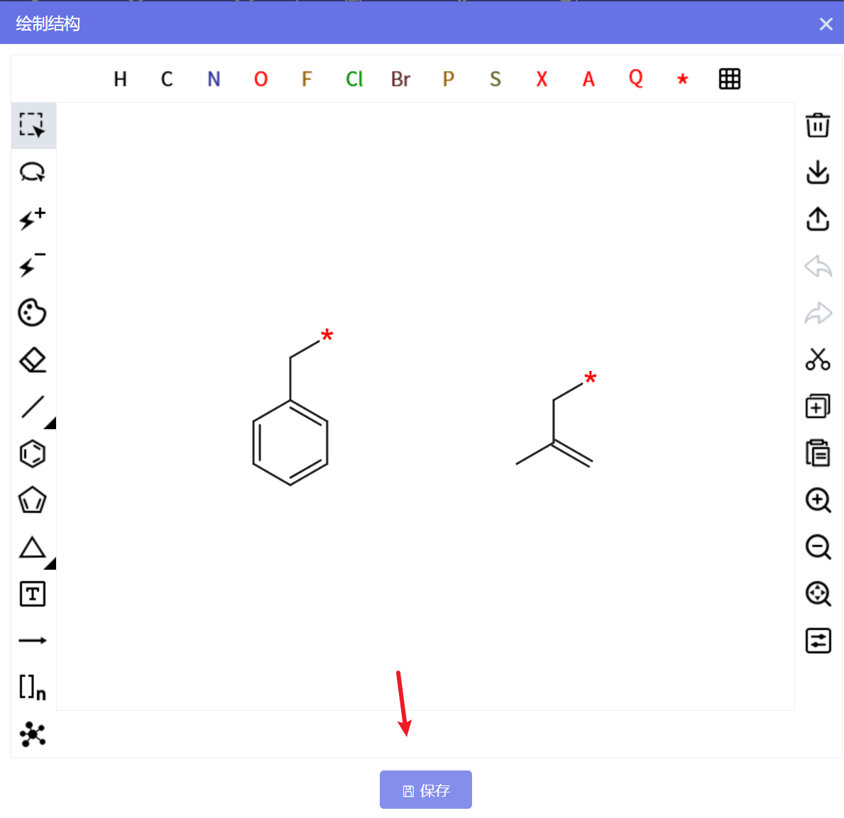
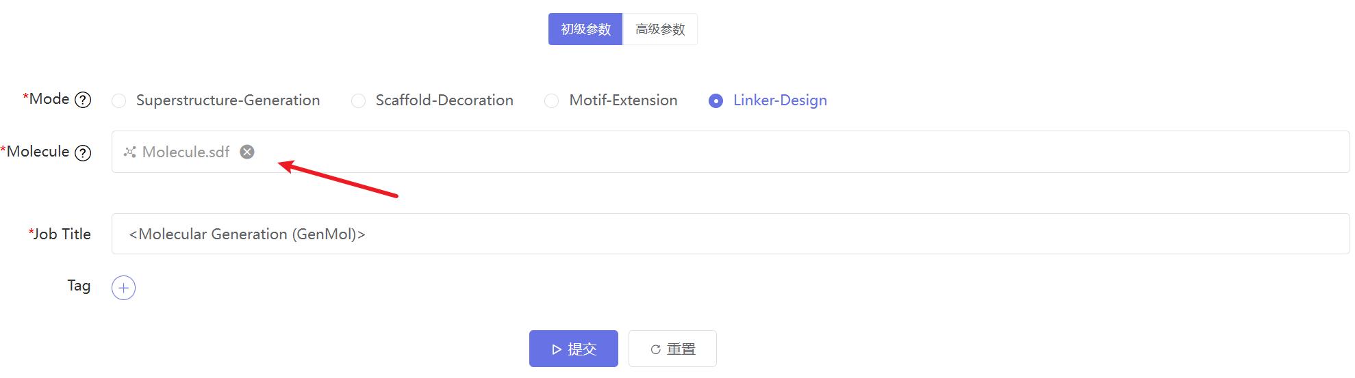
该参数用于指定生成候选样本的数量。程序会按照该大小进行采样,随后自动过滤掉不符合设定片段拼接规则或子结构匹配要求的结果。因此,最终输出的有效样本数可能少于设定值。
采样随机性因子,推荐范围 0–10;数值越低结果越稳定,数值越高结果越多样。
输出文件名称
生成符合要求的结果文件,result.sdf。
GenMol is an open-source AI framework for molecular generation based on a diffusion model. It learns from large chemical databases to generate drug-like molecules. GenMol can simultaneously optimize multiple properties (such as drug-likeness and synthetic accessibility) and provide synthesis planning, roughly ensuring that the generated molecules can be synthesized in a laboratory.
GenMol supports multiple generation modes to meet different drug discovery needs:

Select the generation mode: Superstructure-Generation, Scaffold-Decoration, Motif-Extension, Linker-Design
Molecular structure file in SDF or SMILES format, with file extensions .sdf, .sd, or .smi.
* attachment points are required, which can be generated using the wedraw tool.This parameter specifies the number of candidate molecules to generate. The program will sample according to this value, and then automatically filter out those that do not meet the defined fragment linking rules or substructure matching requirements. Therefore, the final number of valid outputs may be smaller than the specified value.
Sampling randomness factor, recommended range 0–10.
Lower values lead to more stable results, while higher values produce more diverse outputs.
Name of the output file.
Generates the result file result.sdf containing the molecules that meet the specified requirements.
基于受体的结合口袋生成小分子配体。模块基于DiffSBDD模型实现,DiffSBDD于2024年发布,是近年来结构基础药物设计(SBDD)与生成式分子建模领域的代表性进展之一。模型充分利用了SE(3)-等变三维条件扩散模型的最新思想,将蛋白质结合口袋的几何结构直接作为条件输入,结合去噪扩散概率模型(DDPM),能够高效、灵活地生成与目标口袋空间匹配、具有潜在高亲和力的小分子候选物。相较于传统的对接筛选和先导优化方法,该模块可一次性输出多个具备合理构象、较高类药性(QED)和良好合成可行性的分子,显著降低了候选物设计的时间与人工偏差。
DiffSBDD在多个基准数据集上的效果超过以往方法,如下图所示
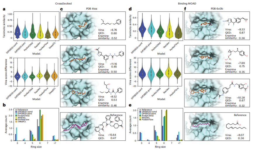
该模块支持多种分子生成场景,助力用户在从头设计(de novo design)、子结构修复(fragment growing & linking)、骨架跃迁(scaffold hopping)等典型药物设计任务中快速获得高价值候选分子。
设计模式,共有四种不同模式可选:
Denovo:从头生成,以复合物结构中的初始配体所在位置作为结合位点,从头生成一批新的配体分子。
Inpaint:配体补全,以复合物结构中的初始配体作为结构增长起点,继续增长结构进一步占据结合位点。
LinkerGen:链接片段生成,以复合物结构中两个配体片段为基础,自动进行链接片段的生成,将两个配体片段进行连接。注意:该模式下,复合物结构中必须存在且仅有两个结构片段位于结合位点。
Optimize:配体性质优化,对复合物结构中的初始配体进行性质优化,两类可选性质。
蛋白与配体小分子的复合物结构文件,PDB格式。小分子所在的结合位置即新分子生成的位置。建议先使用 protein preparation 功能对非标准残基等进行优化
要生成的分子数量,默认为20,最大为1000。
输出文件名称,默认为mols_gen.sdf。
Inpaint模式参数,指定补全过程中需要添加的新原子数量,默认为10。
Optimize模式参数,指定优化的分子性质,可选 sa(合成可行性)或 qed(类药性),默认值为sa。
生成配体分子的结构文件mols_gen.sdf,包含多个分子,分子坐标是复合物中的配体坐标。
Optimize模式下,SDF文件中包含打分信息:
| 列名 | 说明 |
|---|---|
| Score | 合成可行性或类药性的打分,数值在0-1之间,越大表示相应的性质越优 |
This module generates small-molecule ligands based on the binding pocket of a receptor. It is implemented using the DiffSBDD model, which was released in 2024 and represents a major advancement in the field of structure-based drug design (SBDD) and generative molecular modeling. The model leverages the latest developments in SE(3)-equivariant 3D conditional diffusion models by taking the geometric structure of the protein binding pocket as direct input conditions. Combined with a denoising diffusion probabilistic model (DDPM), DiffSBDD can efficiently and flexibly generate small molecules that spatially match the target pocket and have potentially high binding affinity.
Compared to traditional docking-based screening and lead optimization methods, this module can generate multiple candidate molecules in one go—each with reasonable conformations, high drug-likeness (QED), and good synthetic accessibility—greatly reducing design time and human bias.
DiffSBDD outperforms previous methods across multiple benchmark datasets, as shown in the figure below:

This module supports various molecular generation scenarios, helping users quickly obtain high-value candidate compounds for tasks such as de novo design, fragment growing & linking, and scaffold hopping.
Design mode—four different modes are available:
The complex structure file of the protein and ligand in PDB format. The position of the small molecule defines where new molecules will be generated.
It is recommended to use the protein preparation function to clean non-standard residues beforehand.
Number of molecules to generate. Default is 20; maximum is 1000.
Name of the output file. Default is mols_gen.sdf.
Parameter for Inpaint mode. Specifies how many new atoms to add during the completion process. Default is 10.
Parameter for Optimize mode. Specifies the molecular property to optimize:
Options are sa (synthetic accessibility) or qed (drug-likeness).
Default is sa.
The generated ligand structures are saved in an .sdf file named mols_gen.sdf, containing multiple molecules whose coordinates align with the ligand in the complex.
In Optimize mode, an additional score information is included in SDF file, containing:
| Column Name | Description |
|---|---|
| Score | Score for synthetic accessibility or drug-likeness (ranging from 0 to 1; higher is better) |
将DNA序列转换为可视化图像,通过将DNA碱基序列映射到数值并按照核小体(nucleosome)排列模式组织成图像,最终生成彩色图像以直观展示DNA序列的结构特征。功能特点:
物种的基因组序列,FASTA格式
输出图片文件的名称
生成彩色图片,默认名称:genome_visualization.png
This tool converts DNA sequences into visual images by mapping DNA bases to numerical values and organizing them according to the nucleosome arrangement pattern. The result is a colorful image that intuitively displays the structural features of the DNA sequence.
The genome sequence of the species in FASTA format
The name of the output image file
A colorful image is generated with the default file name: genome_visualization.png
将分子结构转换为图片,并显示原子编号。
分子结构文件,格式为SDF或SMILES,文件后缀为.sdf/.sd或.smi
输出图片名称,默认为mol.png
标注了原子编号的分子结构图片。
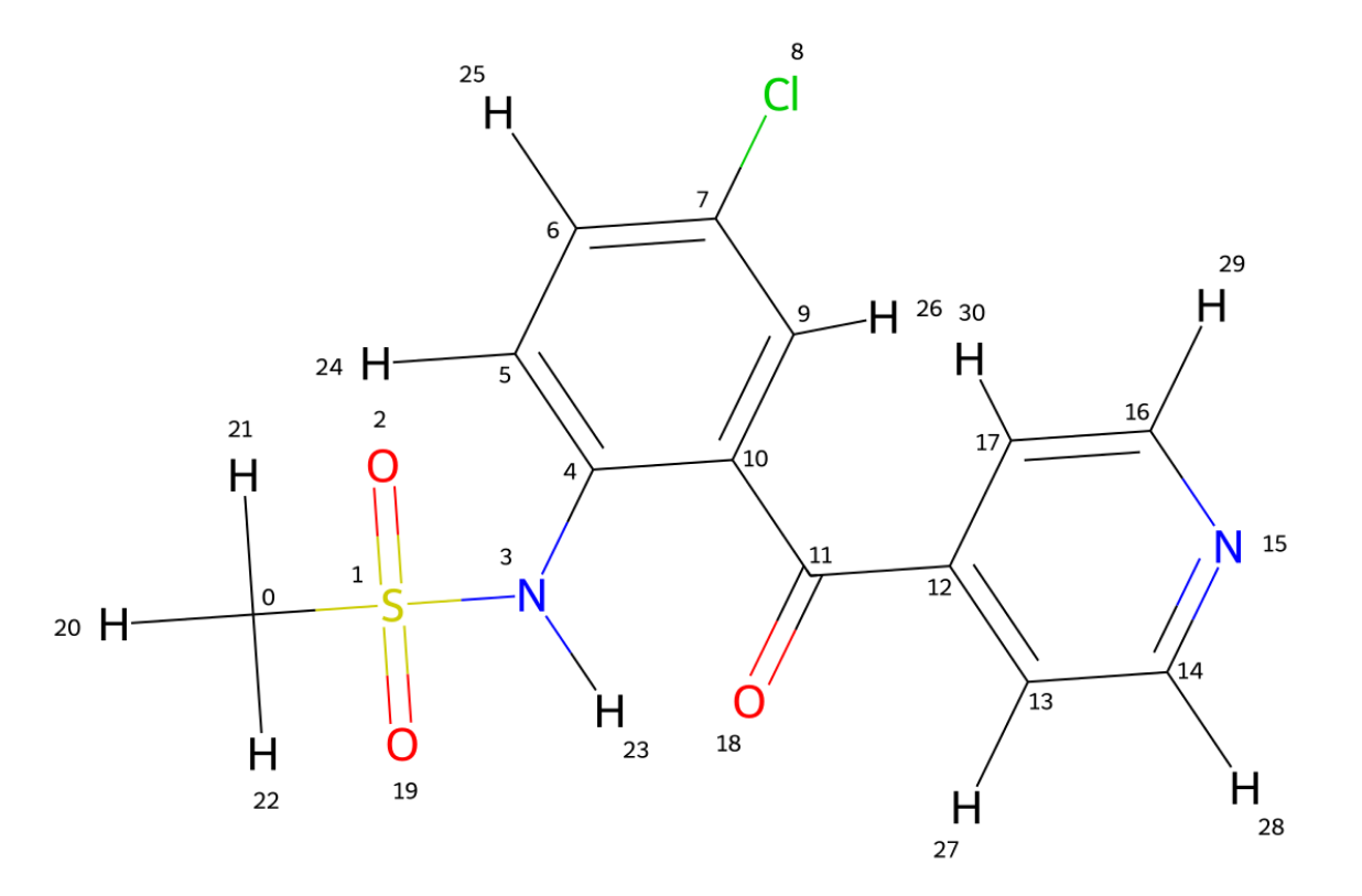
Converts a molecular structure into an image with atom indices labeled.
Molecular structure file in either SDF or SMILES format.
Name of the output image file. Default is mol.png.
An image of the molecular structure with atom indices labeled.

蛋白二级结构残基数目计算。使用 DSSP 算法(即通过检测氨基酸残基之间特定的氢键模式)来确定蛋白质的二级结构。
MD模拟后得到的路径文件,可以在GMX MD Run模块或者AlphaAutoMD模块中获取。
选择需要计算的结构组别:Backbone,Protein,DNA,RNA,Complex。
可以根据PDB中小分子的名称填写组别名称。
注:其中Complex指的是蛋白-小分子复合物体系。
自定义需要计算的残基编号,连续参数可用“-”表示,不连续残基用逗号隔开,例如:1-10,15。
参考md.gro的残基编号。
自定义需要计算的原子编号,连续参数可用“-”表示,不连续残基用逗号隔开,例如:1-10,15。
每一帧的间隔时间(单位ns)
得到结果文件,每种类型的文件如果包含PNG、CSV以及XVG后缀,相同名称只是表现形式不同,数据一样
| 输出文件名称 | 说明 |
|---|---|
| num.xvg/.png/.csv | 不同形式的二级结构的残基数目 |
| ss.png | 每一帧每个残基的二级结构显示文件 |
Calculation of the number of residues in protein secondary structures. The DSSP algorithm determines the secondary structure of proteins by identifying specific hydrogen bonding patterns between amino acid residues.
The trajectory file obtained after MD simulation. This can be retrieved from the GMX MD Run module or the AlphaAutoMD module.
Select the structural group for calculation: Backbone, Protein, DNA, RNA, or Complex.
You can also specify the group name based on the small molecule names in the PDB file.
Note: “Complex” refers to protein-small molecule complex systems.
Specify the residue numbers to analyze. Use a hyphen (-) for continuous ranges and commas (,) for discontinuous residues.
Example: 1-10,15
Refer to the residue numbering in md.gro
Specify the atom numbers to analyze. Use a hyphen (-) for continuous ranges and commas (,) for discontinuous atoms.
Example: 1-10,15
Time interval (in nanoseconds) between each frame.
The result files include the number of residues in different types of secondary structures.
Each type of result may be available in PNG, CSV, and XVG formats. These files have the same content, just different representations.
| Output File Name | Description |
|---|---|
| num.xvg/.png/.csv | Number of residues for each secondary structure type |
| ss.png | Secondary structure visualization for each residue in each frame |
合并稳定性流程(Pythia,ThermoMPNN,ESMIF)输出的结果。
指定ESMIF的结果文件,csv格式,如:ESMIF_results.csv。
指定Pythia的结果文件,csv格式,如:Pythia_results.csv。
指定ThermoMPNN的结果文件,csv格式,如:ThermoMPNN_results.csv。
结果合并输出的文件名称,默认为merged_results.csv
结果合并输出文件merged_results.csv。
Merge the output results from the stability evaluation pipelines: Pythia, ThermoMPNN, and ESMIF.
Specify the result file from ESMIF in CSV format, e.g., ESMIF_results.csv.
Specify the result file from Pythia in CSV format, e.g., Pythia_results.csv.
Specify the result file from ThermoMPNN in CSV format, e.g., ThermoMPNN_results.csv.
Name of the merged output file. Default is merged_results.csv.
The merged result will be output to the file merged_results.csv.

对不同文件中的序列进行组装,输出满足Boltz2批量预测模式需要的序列格式。
进行序列组装的A文件,组装时的固定序列,FASTA格式
进行序列组装的B文件,组装时的遍历序列,FASTA格式
进行序列组装的C文件,组装时的遍历序列,FASTA格式
组装模式,选中表示对B,C文件中的序列进行交叉组装。具体组装逻辑见下述。
组装逻辑:
读取A文件中的所有序列,依次读取B文件及C文件中的相同顺序的一条序列进行组装。如果B文件与C文件中的序列数量不一致,或者其中一个文件为空时,则超出部分的序列单独与A文件序列进行组装。示例如下:
A文件中有两条序列A1/2,B文件中有三条序列B1/2/3,C文件中有5条序列C1/2/3/4/5,输出组合后的序列为:
>A1_A2_B1_C1
A1:A2:B1:C1
>A1_A2_B2_C2
A1:A2:B2:C2
>A1_A2_B3_C3
A1:A2:B3:C3
>A1_A2_C4
A1:A2:C4
>A1_A2_C5
A1:A2:C5
如果选择交叉组装模式,则对B,C文件中的序列进行交叉组装,输出组合后的序列为:
>A1_A2_B1_C1
A1:A2:B1:C1
>A1_A2_B1_C2
A1:A2:B1:C2
>A1_A2_B1_C3
A1:A2:B1:C3
>A1_A2_B1_C4
A1:A2:B1:C4
>A1_A2_B1_C5
A1:A2:B1:C5
>A1_A2_B2_C1
A1:A2:B2:C1
>A1_A2_B2_C2
A1:A2:B2:C2
......
输出组装后的序列文件combined_seqs.fasta。
Assembles sequences from different files and outputs them in the sequence format required for Boltz2 batch prediction mode.
File A used for sequence assembly, fixed sequence during assembly, in FASTA format.
File B used for sequence assembly, traversal sequence during assembly, in FASTA format.
File C used for sequence assembly, traversal sequence during assembly, in FASTA format.
Assembly mode. If selected, sequences from files B and C will be cross-assembled. The specific assembly logic is described below.
Assembly Logic:
Read all sequences from file A. Then, for each sequence in A, read sequences from files B and C in the same order and assemble them together.
If the number of sequences in files B and C are inconsistent, or if one file is empty, the extra sequences will be assembled individually with the sequences from file A.
For example, if file A contains two sequences A1 and A2, file B contains three sequences B1, B2, and B3, and file C contains five sequences C1, C2, C3, C4, and C5, the output assembled sequences will be:
>A1_A2_B1_C1
A1:A2:B1:C1
>A1_A2_B2_C2
A1:A2:B2:C2
>A1_A2_B3_C3
A1:A2:B3:C3
>A1_A2_C4
A1:A2:C4
>A1_A2_C5
A1:A2:C5
If cross-assembly mode is selected, sequences from files B and C will be cross-assembled. The output sequences will be:
>A1_A2_B1_C1
A1:A2:B1:C1
>A1_A2_B1_C2
A1:A2:B1:C2
>A1_A2_B1_C3
A1:A2:B1:C3
>A1_A2_B1_C4
A1:A2:B1:C4
>A1_A2_B1_C5
A1:A2:B1:C5
>A1_A2_B2_C1
A1:A2:B2:C1
>A1_A2_B2_C2
A1:A2:B2:C2
......
The assembled sequence file will be output as combined_seqs.fasta.
对ESM2蛋白质语言模型进行微调,支持分类(二分类)和回归任务。
该模块提供了四种训练方法:
1,基于BioNeMo框架的全参微调
2,基于BioNeMo框架的LoRA(Low-Rank Adaptation)参数高效微调。
3,序列特征迁移+传统机器学习(ML)预测头
4,序列特征迁移+多层感知机(MLP)预测头
默认会尝试所有训练方法,自动比较训练结果并选择最佳模型。训练完成后可基于训练后的最佳模型进行推理。
训练
训练方法:All (所有方法)、Finetune (基于 BioNeMo 框架的全参微调)、Lora(基于 BioNeMo 框架的 LoRA 参数高效微调)、Ml (序列特征迁移 + 传统机器学习预测头)、MLP (序列特征迁移 + 多层感知机预测头)。
用于训练的数据文件路径,CSV 格式(逗号分隔的文本文件格式)。
数据文件中蛋白序列所在列的列名称,如 “sequence”。
数据文件中标签所在列的列名称,如 “label”,标签可以是序列的性质(如:亲和力、稳定性等),也可以是类别(0 或 1 等)。
任务类型:classification 或 regression。
训练数据中用于作为测试集的比例,默认值 0.2。
训练轮次,默认 10。
训练时的批次大小,默认 16。
推理
用于推理的数据文件路径。支持以下格式:
当输入为 CSV 格式时,指定序列所在列的列名称,如“sequence”。
如未指定,将自动从 model_info_file 中读取训练时使用的列名称,此时需确保推理数据文件中的列名称与训练数据一致。
当输入为 FASTA 格式时,无需填写该参数。
模型信息 JSON 文件路径(训练任务最终输出的 result.json 文件)。
推理结果筛选方式:largest(由大到小排序)、smallest(由小到大排序)、closest(按最接近某个数值排序,仅适用于回归任务)。
筛选保留的样本数量,默认值 10000。
如果选择 closest 模式,需要指定的目标值。
对于分类任务,只保留特定类别的样本。
result.json:模型信息文件,包含任务ID、方法、模型路径等信息methods_comparison.csv:不同方法的性能比较结果| 指标 | 说明 |
|---|---|
| Spearman | Spearman相关性指标,-1至1之间,绝对值越大表示相关性越高,模型效果越好。不同训练方法得到回归模型通过该参数进行排序,选取最优模型。 |
| MAE | 平均绝对误差,数值越小越好 |
分类任务的模型评价指标:
| 指标 | 说明 |
|---|---|
| Accuracy | 准确率,整体预测正确的比例,0-1之间,越大表示模型效果越好 |
| Precision | 精确率,预测为正例的样本中,实际为正的比例,0-1之间,越大表示模型效果越好 |
| Recall | 召回率,实际为正例的样本中,被正确预测的比例,0-1之间,越大表示模型效果越好 |
| F1_score | 精确率与召回率的调和平均值。不同训练方法得到分类模型通过该参数进行排序,选取最优模型。 |
train_report.pdf:各方法的性能结果报告(PDF格式)注意:当训练模型失败或指标不符合要求时(如:Spearman为0),不输出该模型及其指标。
predictions.csv:预测结果文件,输出序列及预测打分(与训练数据中label列的性质一致)。This module is designed for fine-tuning the ESM2 protein language model, supporting classification (binary) and regression tasks. It offers three training methods:
By default, all training methods are attempted, and the results are automatically compared to select the best model. After training, inference can be performed using the best-trained model.
Training strategy. Supported options:
Path to the training dataset file.
Only CSV format (comma-separated values) is supported.
Name of the column containing protein sequences in the dataset (e.g., sequence).
Name of the column containing labels in the dataset (e.g., label).
Labels can represent:
Type of task:
Proportion of the dataset used as the test set.
Default: 0.2
Number of training epochs.
Default: 10
Batch size used during training.
Default: 16
Path to the input file for inference. Supported formats:
Required when the input file is in CSV format, specifying the column name that contains the sequences,such as “suquence”.
If not provided, the column name will be automatically loaded from model_info_file, and must match the column used during training.
This parameter is not required when using FASTA format.
Path to the JSON file containing model metadata (i.e., result.json generated during training).
Method used to filter and rank inference results:
Number of samples to retain after filtering.
Default: 10,000
Required when using closest mode.
Specifies the target value for ranking.
Used in classification tasks to retain samples belonging to a specific class.
result.json: Model information file, including task ID, method, model path, etc.methods_comparison.csv: Performance comparison results of different methods.Model Evaluation Metrics for Regression Tasks:
| Metric | Description |
|---|---|
| Spearman | Spearman correlation coefficient, ranging from -1 to 1. A higher absolute value indicates stronger correlation and better model performance. Regression models from different training methods are ranked based on this metric to select the optimal model. |
| MAE | Mean Absolute Error. Smaller values indicate better performance. |
Model Evaluation Metrics for Classification Tasks:
| Metric | Description |
|---|---|
| Accuracy | Proportion of correct predictions overall, ranging from 0 to 1. Higher values indicate better model performance. |
| Precision | Proportion of true positives among predicted positives, ranging from 0 to 1. Higher values indicate better performance. |
| Recall | Proportion of true positives correctly identified, ranging from 0 to 1. Higher values indicate better performance. |
| F1_score | Harmonic mean of precision and recall. Classification models from different training methods are ranked based on this metric to select the optimal model. |
train_report.pdf: Performance reports for each method (in PDF format).Note: If model training fails or evaluation metrics do not meet requirements (e.g., Spearman = 0), the model and its metrics will not be included in the output.
predictions.csv: File containing predicted sequences and their corresponding prediction scores (same to the label column properties in the training data)Mutation Score是抗体人源化设计中核心模块,是一个基于结构的自动化评分模块。该模块基于抗体的结构信息以及CDR嫁接后的序列信息,对移植抗体(graft)后的FR区的每个氨基酸在替换前后的变化程度进行量化评分。评分越高,说明CDR嫁接过程中氨基酸的替换对CDR区的构象可能影响较大,需要进行回复突变。模块输出每个氨基酸的打分值,用于抗体人源化设计流程中后续的分组和人源化抗体序列的生成。
抗体Fv区序列文件,FASTA格式。
抗体结构文件,PDB格式。
抗体CDR区Graft后的序列文件,FASTA格式。
抗体FR区序列比对结果文件,FASTA格式
界面相互作用计算结果,包含原子/残基级别的接触信息
氢键计算结果,包含供体-受体对、距离和角度信息
指定输出打分文件的名称,CSV格式。
抗体类型:
抗体编号规则:kabat,imgt,chothia
输出结果文件为score.csv,包含信息如下:
| 字段名称 | 说明 |
|---|---|
| Chain | 轻链或重链 |
| UID | 为残基的标准编号(默认为 Kabat) |
| Position | 残基在序列中的位置 |
| Donor Residue | 原始氨基酸 |
| Template Residue | 人源模板的目标氨基酸 |
| score | 回复突变智能评分,Score 越高,认为其回复突变的必要性越高。通常Score>10为高优先级,5-10为中优先级,其他为低优先级 |
Mutation Score is a core module in antibody humanization design, serving as a structure-based automated scoring module. This module quantitatively scores the degree of change for each amino acid in the FR region after grafting CDRs based on the antibody’s structure and the sequence information post-CDR grafting. A higher score indicates that the replacement of amino acids during CDR grafting may have a significant impact on the CDR region’s conformation, suggesting the need for revertant mutations. The module outputs a score for each amino acid, which is used in subsequent grouping and generation of humanized antibody sequences in the antibody humanization design process.
Sequence file of the antibody Fv region in FASTA format.
Antibody structure file in PDB format.
Sequence file of the antibody CDR region after grafting in FASTA format.
Specify the name of the output scoring file in CSV format.
Interface interaction calculation results, including atom/residue-level contact information
Interface interaction calculation results, including atom/residue-level contact information
Type of antibody:
Antibody numbering type: kabat,imgt,chothia
The output result file is named score.csv and includes the following information:
| Field Name | Description |
|---|---|
| Chain | Light chain or heavy chain |
| UID | Standard numbering for residues (default is Kabat) |
| Position | Position of the residue in the sequence |
| Donor Residue | Original amino acid |
| Template Residue | Target amino acid from the human template |
| Score | Revertant mutation intelligence score, where a higher score suggests a higher necessity for a revertant mutation. Typically, a Score > 10 is high priority, 5-10 is medium priority, and others are low priority. |
.png)
LocalRetro 是局部逆合成预测框架,其动机是化学直觉认为分子变化主要发生在化学反应过程中的局部。这与几乎所有现有的逆合成方法不同,这些方法根据分子的全局结构建议反应物,通常包含与反应没有直接关系的精细细节。这个局部概念产生了涉及原子和键编辑的局部反应模板。由于远程官能团也可以作为次要方面影响整个反应路径,因此进一步细化了所提出的局部编码逆合成模型,以通过全局注意力机制来解释化学反应的非局部效应。模型显示,对于包含 50016 个反应的 USPTO-50K 数据集,top-1 名和 top-5 预测的准确率分别为 89.5% 和 99.2%。在包含 479035 个反应(UTPTO-MIT) 的大型数据集上 top-1 和 top-5 准确率分别为 87.0% 和 97.4%。通过从各种文献中正确预测五种候选药物分子的合成途径,还证明了该模型的实际应用。

输入小分子的SMILES,支持多个批量预测,一行一个,示例:
O=C(Nc4cccc(C(=O)N3CCN(c1ccnc2[nH]ccc12)C3)c4)c5cccc(C(F)(F)F)c5
输出的CSV文件包含以下列:
| 列名 | 说明 |
|---|---|
Input SMILES |
输入的原始分子SMILES |
Predicted Reactants |
预测反应物的SMILES |
Predicted Site |
预测的反应位点 |
Local Reaction Template |
局部反应模板 |
Score |
预测得分,范围0-1,分数越高,表明该反应发生概率越高 |
注意: 每个输入分子可能产生多个预测反应,因此一个分子会对应多行数据。
LocalRetro, a local retrosynthesis framework, motivated by the chemical intuition that the molecular changes occur mostly locally during the chemical reactions. This differs from nearly all existing retrosynthesis methods that suggest reactants based on the global structures of the molecules, often containing fine details not directly relevant to the reactions. This local concept yields local reaction templates involving the atom and bond edits. Because the remote functional groups can also affect the overall reaction path as a secondary aspect, the proposed locally encoded retrosynthesis model is then further refined to account for the nonlocal effects of chemical reaction through a global attention mechanism. Model shows a promising 89.5 and 99.2% round-trip accuracy at top-1 and top-5 predictions for the USPTO-50K dataset containing 50 016 reactions. LocalRetro was further validated on a large dataset containing 479 035 reactions (UTPTO-MIT) with comparable round-trip top-1 and top-5 accuracy of 87.0 and 97.4%, respectively. The practical application of the model is also demonstrated by correctly predicting the synthesis pathways of five drug candidate molecules from various literature.
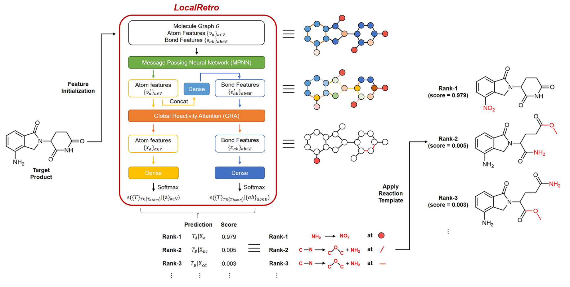
SMILES of small molecules, supporting batch prediction of multiple entries, one per line. Demo:
O=C(Nc4cccc(C(=O)N3CCN(c1ccnc2[nH]ccc12)C3)c4)c5cccc(C(F)(F)F)c5
Output CSV file includes:
| Column Name | Description |
|---|---|
Input SMILES |
input SMILES for prediction |
Predicted Reactants |
Predicted reactant in SMILES |
Predicted Site |
Predicted reaction site |
Local Reaction Template |
Template used |
Score |
Predicted score(0~1),and a high score indicating higher the likelihood of the reaction. |
Note: Each input molecule may generate multiple predicted reactions, so one molecule may correspond to multiple lines of data
预测小分子与蛋白的亲和力(用pIC50表示)。模块基于DeepPurpose框架实现,采用的预训练模型为MPNN_CNN_BindingDB,是基于BindingDB数据库训练的小分子-蛋白亲和力预测模型。
模型架构如图所示:
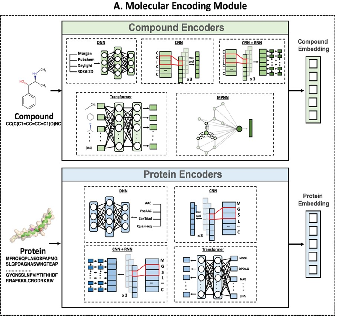
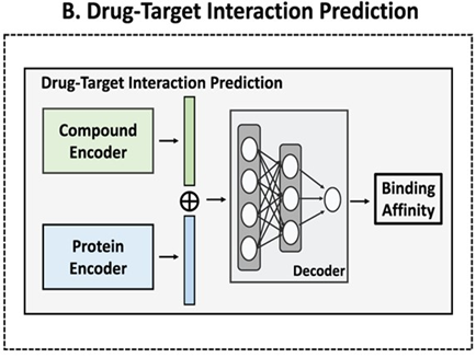
模型预测效果在当时是最佳的:
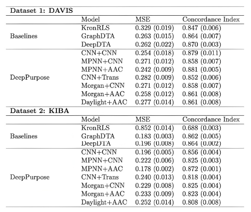
单个或多个蛋白序列,FASTA格式或TXT格式,每个蛋白使用一条序列表示(有多条链时,将单链序列收尾连接放在同一条序列中),txt格式时,每行一个蛋白。
小分子结构文件,TXT格式,支持多个底物分子,使用SMILES表示,每行一个分子,文件内容示例:
OC1=CC=C(C[C@@H](C(O)=O)N)C=C1
CC(O)O
注意:
输入每个小分子都会与每个蛋白计算亲和力,并输出结果。
亲和力预测结果文件名,默认为pred_res.csv
结果文件pred_res.csv,包含以下信息:
| 列名 | 说明 |
|---|---|
| SMILES | 小分子结构 |
| Target_ID | 蛋白名称 |
| Target_Sequence | 蛋白序列 |
| Score(pIC50) | 预测的亲和力pIC50数值,越大表示亲和力越高,可与阳性对照分子的预测数值比较。 |
This module predicts the binding affinity between small molecules and proteins, expressed as pIC50. It is implemented based on the DeepPurpose framework, using the pre-trained model MPNN_CNN_BindingDB, which was trained on the BindingDB dataset for small molecule–protein affinity prediction.
The model architecture is shown below:
At the time of its release, the model achieved state-of-the-art performance:
One or more protein sequences in FASTA or TXT format. Each protein should be represented by a single sequence. For multi-chain proteins, concatenate the chain sequences end-to-end into one line. In TXT format, each line represents one protein.
Small molecule structure file in TXT format, supporting multiple substrate molecules. Molecules are represented using SMILES, with one molecule per line. Example content:
OC1=CC=C(C[C@@H](C(O)=O)N)C=C1
CC(O)O
Note:
Each small molecule will be paired with each protein to compute the binding affinity, and the results will be output accordingly.
The output filename for affinity prediction results. Default is pred_res.csv.
The result file pred_res.csv contains the following fields:
| Column Name | Description |
|---|---|
| SMILES | Small molecule structure (SMILES format) |
| Target_ID | Protein name |
| Target_Sequence | Protein sequence |
| Score (pIC50) | Predicted binding affinity score (pIC50). A higher value indicates stronger binding, and can be compared with positive control molecules. |
对蛋白、抗体序列进行聚类、可视化。模块使用MMseq2算法对序列进行聚类分析,将多序列分为多个cluster类别,并通过ESM2模型对序列进行embedding,通过可视化模块UMAP对序列embedding进行降维,获取二维可视化信息。
蛋白或抗体序列,FASTA格式
聚类中采用的最小序列一致性数值,范围在0-1之间,默认值为0.5,表示至少具有50% identity的序列才会被聚为一类。
序列类型,选中表示抗体序列,否则为蛋白序列。
序列类型为抗体时的编号规则,支持imgt, chothia, kabat
序列聚类方案,支持2种:full, cdr(仅序列类型为抗体时可用)。‘full’表示使用全长序列进行聚类,‘cdr’表示使用CDR序列进行聚类(具体CDR位置在参数‘CDRs’中设定),默认为‘full’
指定用于聚类的CDR区域,在‘Cluster’参数为cdr时生效。可选区域为(支持多选):CDR1,CDR2,CDR3。默认选择CDR3。
输出cluster_res.csv结果文件,包含以下信息:
| 列名 | 说明 |
|---|---|
| ID | 序列名称 |
| Sequence | 序列 |
| CDR1_AA | CDR1的氨基酸序列,序列为抗体时输出 |
| CDR2_AA | CDR2的氨基酸序列,序列为抗体时输出 |
| CDR3_AA | CDR3的氨基酸序列,序列为抗体时输出 |
| Cluster_ID | 序列所属类别编号,从1开始按顺序编号 |
| Cluster_Size | 序列所属类别包含的序列数目,如:‘5’表示该类别含有5条序列 |
| Cluster_Center | 序列是否为聚类中心,'1’表示是,‘0’表示不是 |
Cluster and visualize protein and antibody sequences. This module uses the MMseqs2 algorithm to perform clustering analysis on sequences, dividing multiple sequences into several cluster categories. It uses the ESM2 model to embed the sequences, and the visualization module UMAP to reduce the dimensionality of the sequence embeddings, obtaining two-dimensional visualization information.
Protein or antibody sequences in FASTA format.
The minimum sequence identity value used in clustering, ranging from 0 to 1. The default value is 0.5, which means sequences must have at least 50% identity to be clustered together.
The type of sequence. Selecting indicates antibody sequences; otherwise, it is protein sequences.
The numbering scheme for antibody sequences, supporting imgt, chothia, kabat.
Sequence clustering scheme, supporting two types: full and cdr (only available for antibody sequences). ‘full’ means using the full-length sequence for clustering, while ‘cdr’ means using CDR sequences for clustering (specific CDR positions are set in the ‘CDRs’ parameter). The default is ‘full’.
Specifies the CDR regions used for clustering, effective when the ‘Cluster’ parameter is set to cdr. Optional regions (supporting multiple selections) are: CDR1, CDR2, CDR3. The default selection is CDR3.
Outputs a result file named cluster_res.csv containing the following information:
| Column Name | Description |
|---|---|
| ID | Sequence name |
| Sequence | Sequence |
| CDR1_AA | Amino acid sequence of CDR1, output when the sequence is an antibody |
| CDR2_AA | Amino acid sequence of CDR2, output when the sequence is an antibody |
| CDR3_AA | Amino acid sequence of CDR3, output when the sequence is an antibody |
| Cluster_ID | Cluster category number of the sequence, numbered sequentially starting from 1 |
| Cluster_Size | Number of sequences in the cluster category, e.g., ‘5’ means the category contains 5 sequences |
| Cluster_Center | Whether the sequence is a cluster center, ‘1’ indicates yes, ‘0’ indicates no |
该模块是抗体人源化设计流程中分组模块,根据Mutation Score模块输出的回复突变评分表对回复突变进行分组。
更新内容:
抗体CDR区嫁接后序列文件,FASTA格式,由Grafting模块生成
抗体序列文件,FASTA格式
人源化突变评分文件,CSV格式,由Mutation Score模块生成
指定输出的突变序列文件名称,FASTA格式
打分分组的截断值,逗号分割,例如:2,5,10表示将氨基酸突变评分大于10的为一组,5~10的氨基酸为一组,小于2的氨基酸分为一组。如果是纳米抗体,控制数量为 3 个,三个cutoff划分成4组:第一组仅T1,第二组开始T1全部+T2中一个轮换,第三组加入全部T2,第四组加入全部T3
指定输出的回复突变的文件
普通抗体Antibody或者纳米抗体Nanobody
抗体CDR区嫁接后序列文件,FASTA格式,由Grafting模块生成
抗体序列文件,FASTA格式
人源化突变评分文件,CSV格式,由Mutation Score模块生成
指定输出的突变序列文件名称,FASTA格式
打分分组的截断值,逗号分割,例如:2,5,10表示将氨基酸突变评分大于10的为一组,5~10的氨基酸为一组,小于2的氨基酸分为一组。如果是纳米抗体,控制数量为 3 个,三个cutoff划分成4组:第一组仅T1,第二组开始T1全部+T2中一个轮换,第三组加入全部T2,第四组加入全部T3
指定输出的回复突变的文件
普通抗体Antibody或者纳米抗体Nanobody
突变组合的截断值,Mutation Score模块中输出的氨基酸回复突变打分大于截断值的氨基酸参与生成突变组合
高于截断值的突变自动进行回复突变
每条链回复突变打分在Combination Min Cutoff与Combination Max Cutoff之间的选择打分前n个位置进行组合突变
根据不同截断值得到突变分组结果文件mutate_policy.json。
高通量方法HTS Mutate中根据组合突变截断值得到的突变分组结果文件combination_mutate_policy.json,高通量人源化设计流程。
Back mutation grouping in the antibody humanization, which groups the back mutations based on the mutation scoring table generated by the Mutation Score module.
Update Log:
Sequence file of the antibody CDR region after grafting, in FASTA format, generated by the Grafting module.
Sequence file of the antibody, in FASTA format.
Humanization mutation score file, in CSV format, generated by the Mutation Score module.
Specify the name of the output mutation sequence file, in FASTA format.
The cutoff values for score-based grouping, separated by commas. For example, “2,5,10” means: amino acid mutations with scores >10 are grouped together, those with scores between 5 and 10 form one group, and those with scores <2 form another group. For nanobodies, control the number to 3. Three cutoffs divide into 4 groups: the first group contains only T1; the second group includes all of T1 plus one rotation from T2; the third group adds all of T2; the fourth group adds all of T3.
Specify the file for the output of back mutations.
Antibody or Nanobody
Cutoff value for mutation combinations. Amino acids with scores (generated from Mutation Score module) greater than the cutoff value are involved in the mutation combinations.
Mutations above the cutoff value automatically undergo reversion mutations.
For each chain, select the top n positions with back mutation scores between the Combination Min Cutoff and the Combination Max Cutoff for combination mutations.
The mutation grouping results file mutate_policy.json is generated based on different cutoff values.
In HTS Mutate, the mutation grouping results file combination_mutate_policy.json is generated based on combination cutoff values.
Humanization Report v2.5是抗体人源化设计报告生成模块,用于生成最终的抗体人源化设计报告以及相应的专利实施例段落。
更新日志:
Grafting模块生成的Graft Policy文件。
Back Mutation Grouping模块生成的Policy文件。
抗体类型,Antibody 标准双链抗体,Nanobody 纳米抗体。
Grafting模块生成的score文件,JSON格式
Mutation模块生成的score文件,CSV格式
Grafting模块生成的Graft Policy文件。
Back Mutation Grouping模块生成的Policy文件。
抗体类型,Antibody 标准双链抗体,Nanobody 纳米抗体。
Grafting模块生成的score文件,JSON格式
Mutation模块生成的score文件,CSV格式
抗体结构RMSD文件,由Antibody RMSD模块生成,CSV格式
从RMSD排序中取前N个RMSD值小的抗体
Absolute Folding Stability模块预测生成的蛋白稳定性文件,CSV格式
输出结果包括:
| 输出文件名称 | 说明 |
|---|---|
| BM.pptx | 回复突变位点汇总文件 |
| batch_registration_template.xlsx | 批量注册模板文件 |
| hotspot_summary.xlsx | 风险位点总结 |
| patent_example_template.docx | 人源化设计序列在相应的专利实施例段落 |
| patent_example_en_template.docx | 英文版人源化设计序列在相应的专利实施例段落 |
| back_mutation_grouping.md | 回复突变分组信息 |
| candidate_score.xlsx | 人源化抗体序列的结构和能量打分汇总 |
| humanized_variants.fasta | 抗体人源化设计序列文件,FASTA格式 |
| Report.docx | 抗体人源化设计报告,包括整个人源化设计过程涉及的序列、分组等信息 |
其中batch_registration_template.xlsx包含如下信息:
| 字段名称 | 说明 |
|---|---|
| Protein Sequence | 蛋白序列 |
| Molecule Name | 分子名称 |
其中hotspot_summary.xlsx包含如下信息:
| 字段名称 | 说明 |
|---|---|
| ID | 抗体序列名称 |
| Sequence-CDR | CDR序列区域 |
| Deamidation | 脱酰胺位点 |
| Isomerization | 异构化位点 |
| Cleavage | 酶切位点 |
| Hydrolysis | 水解位点 |
| Glycosylation | 糖基化位点 |
| Cys | 半胱氨酸数量 |
| Oxidation | 氧化位点 |
| High risk | 高风险率 |
| High risk sites | 高风险位点 |
The Humanization Report v2.5 is a module for generating reports on antibody humanization design, including the final antibody humanization design report and corresponding paragraphs for patent implementation examples.
Update Log:
The Graft Policy file generated by the Grafting module.
The Policy file generated by the Back Mutation Grouping module.
Antibody type, Antibody or Nanobody
Graft germline score file in JSON format generated by the Grafting module
Mutation score file in csv format generated by the Mutation module
The Graft Policy file generated by the Grafting module.
The Policy file generated by the Back Mutation Grouping module.
Antibody type, Antibody or Nanobody
Graft germline score file in JSON format generated by the Grafting module
Mutation score file in csv format generated by the Mutation module
Antibody structure RMSD file generated by Antibody RMSD module
Select the top N antibodies with the smallest RMSD values from the RMSD ranking
Protein folding stability file generated by Absolute Folding Stability module in CSV format
The output results include:
| Output File Name | Description |
|---|---|
| BM.pptx | Summary file of back mutation sites |
| batch_registration_template.xlsx | Batch registration template file |
| hotspot_summary.xlsx | Summary of hotspot sites |
| patent_example_template.docx | Humanization design sequences in corresponding patent implementation example paragraphs (Chinese version) |
| patent_example_en_template.docx | Humanization design sequences in corresponding patent implementation example paragraphs (English version) |
| back_mutation_grouping.md | Grouping for back mutations |
| humanized_variants.fasta | Antibody humanization design sequence file in FASTA format |
| Report.docx | Antibody humanization design report, including information on sequences, grouping, etc., involved in the entire humanization design process |
| candidate_score.xlsx | Candidate sequences energy and structure scores |
The batch_registration_template.xlsx file contains the following information:
| Field Name | Description |
|---|---|
| Protein Sequence | Protein sequence |
| Molecule Name | Molecule name |
The hotspot_summary.xlsx file contains the following information:
| Field Name | Description |
|---|---|
| ID | Antibody sequence name |
| Sequence-CDR | CDR sequence region |
| Deamidation | Deamidation site |
| Isomerization | Isomerization site |
| Cleavage | Cleavage site |
| Hydrolysis | Hydrolysis site |
| Glycosylation | Glycosylation site |
| Cys | Number of cysteines |
| Oxidation | Oxidation site |
| High risk | High-risk rate |
| High risk sites | High-risk sites |
合并AF3-like模型(Boltz-2,Protenix,Chai-1)输出的结果。
指定Boltz2结果的打包文件,tar格式,如:Boltz_results.tar。
指定Protenix结果的打包文件,tar格式,如:Protenix_results.tar。
指定Chai-1结果的打包文件,tar格式,如:Chai-1_results.tar。
结构文件合并输出的打包文件名称,默认为merged_results.tar。
打分文件合并输出的打包文件名称,默认为merged_results.csv。
结构文件的合并输出打包文件merged_results.tar,包含输入的所有AF3-like模型预测结果。
打分文件的合并输出打包文件merged_results.csv,包含所有AF3-like模型的打分。
Merge the output results of AF3-like models (Boltz-2, Protenix, Chai-1).
Specify the packaged result file from Boltz-2 in tar format, e.g., Boltz_results.tar.
Specify the packaged result file from Protenix in tar format, e.g., Protenix_results.tar.
Specify the packaged result file from Chai-1 in tar format, e.g., Chai-1_results.tar.
Name of the merged output tar file containing structure files. Defaults to merged_results.tar.
Name of the merged output file containing scores. Defaults to merged_results.csv.
The merged output tar file merged_results.tar contains the structural prediction results from all the input AF3-like models.
The merged score file merged_results.csv includes the scores from all AF3-like models.
合并AF3-like模型打分结果与PPI模块打分结果,并汇总输出。
指定AF3-like多个模型打分的汇总文件,csv格式,如:merged_results.csv。
指定PPI模型Prodigy的结果打分文件,csv格式,如:prodigy_output.csv。
指定PPI模型Graphomer的结果打分文件,csv格式,如:PPI_pred.csv。
打分合并输出的文件名称,默认为score_merge.csv。
打分的合并输出打包文件score_merge.csv,包含所有AF3-like模型的打分及PPI模型打分。
Merge the scoring results from AF3-like models with the PPI module scoring results and generate a consolidated output.
Specify the consolidated score file from multiple AF3-like models in CSV format, e.g., merged_results.csv.
Specify the scoring result file from the PPI model Prodigy in CSV format, e.g., prodigy_output.csv.
Specify the scoring result file from the PPI model Graphomer in CSV format, e.g., PPI_pred.csv.
Name of the merged output score file. Defaults to score_merge.csv.
The merged score output file score_merge.csv includes scoring results from all AF3-like models and PPI models.
该模块预测酶的动力学参数Kcat与Km。模块基于UniKP框架实现,UniKP是一个用于预测酶动力学参数的计算工具。它结合了蛋白质序列和底物结构信息,利用预训练的语言模型(如 ProtT5-XL-UniRef50)来生成酶的表示,并通过深度学习模型预测酶的动力学参数。
UniKP框架由两个关键组件组成:表示模块和机器学习模块。表示模块使用预训练的语言模型对酶和底物的信息进行编码。具体而言,酶序列中的氨基酸使用ProtT5-XL-UniRef50模型转换为1024维的向量。对于每个蛋白质,应用平均池化方法得到其表示,这被发现是对于蛋白质任务最有效的方法。另一方面,底物结构被转换为简化的分子输入线条记录系统(SMILES)格式,并通过预训练的SMILES转换器进行处理,每个符号生成一个256维的向量。然后,对最后一层和倒数第二层的第一个输出进行平均池化和最大池化,将它们连接起来生成一个1024维的分子表示向量。蛋白质和底物的连接表示向量随后被输入到机器学习模块中(整体架构图如下)。
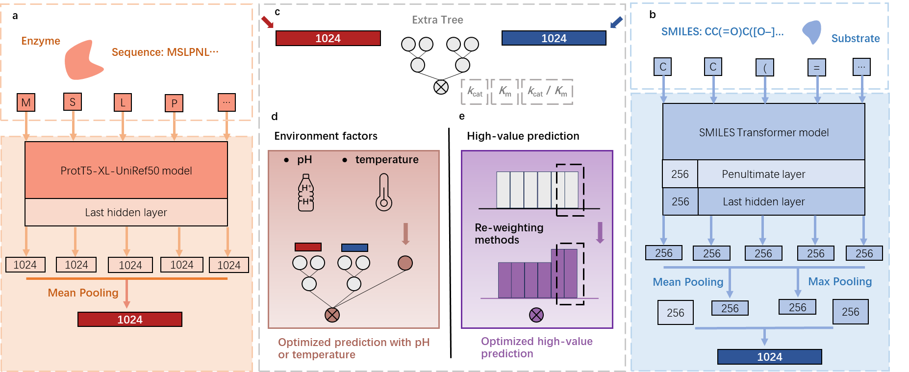
在kcat预测任务中使用DLKcat数据集进行验证。在没有任何额外参数优化的情况下,通过五轮随机分割的测试集上的平均确定系数(R2)值为0.68,比DLKcat提高了20%。此外,这五轮中DLKcat的最高值比UniKP的最低值低16%,进一步证明了UniKP的稳健性。预测值和实验测量值之间的均方根误差(RMSE)在UniKP中也比DLKcat低,无论是在训练集还是测试集中。在测试集中,预测值和实验测量值之间存在着强烈的相关性,相关系数(PCC)为0.85,整个数据集的相关系数为0.99,比DLKcat分别高出14%和11%。
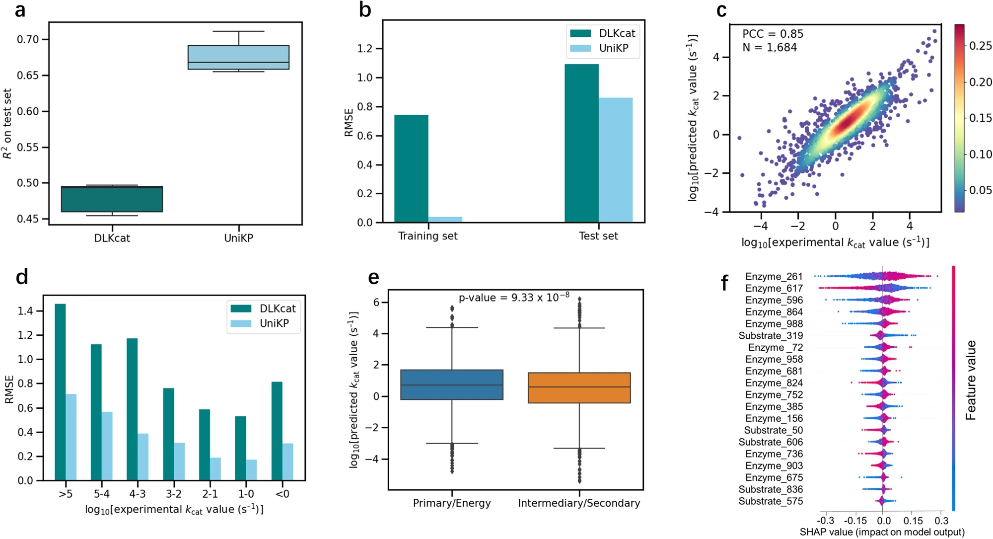
单个或多个酶的序列,fasta格式,每个酶使用一条序列表示(当某个酶有多条链时,将多条单链序列首尾连接作为一条序列)。
底物分子的文件,txt格式,支持多个底物分子,使用SMILES表示,每行一个分子,文件内容示例:
OC1=CC=C(C[C@@H](C(O)=O)N)C=C1
CC(O)O
注意:
1,输入的底物分子数量与酶数量应相同,模块会按文件中的顺序进行酶与底物分子配对。
2,当有多个酶分子时,可只设置一个底物分子,表示每个酶都使用相同的底物分子。
动力学参数预测结果文件名,默认为pred_res.csv
动力学参数结果文件pred_res.csv,包含以下信息:
| 列名 | 说明 |
|---|---|
| SeqID | 序列名称 |
| Sequence | 酶序列 |
| SMILES | 底物分子 |
| Kcat(n/s) | 酶的周转数,是酶的动力学参数之一。表示每个酶分子单位时间内能转化底物的最大分子数,单位为个/秒 |
| Km(mM) | 米氏常数,是另一个酶的动力学参数。代表反应速率为最大反应速率一半时的底物浓度,单位为mM |
This module predicts the kinetic parameters Kcat and Km of enzymes. It is implemented based on the UniKP framework, a computational tool designed for enzyme kinetic parameter prediction. UniKP integrates protein sequence and substrate structure information, utilizing pre-trained language models (such as ProtT5-XL-UniRef50) to generate enzyme representations and employs deep learning models to predict enzyme kinetic parameters.
The UniKP framework consists of two key components: the representation module and the machine learning module. The representation module encodes information of enzymes and substrates using pre-trained language models. Specifically, amino acids in enzyme sequences are transformed into 1024-dimensional vectors using the ProtT5-XL-UniRef50 model. For each protein, average pooling is applied to obtain its representation, which has been found to be the most effective method for protein tasks. On the other hand, substrate structures are converted into Simplified Molecular Input Line Entry System (SMILES) format and processed by a pre-trained SMILES encoder, generating a 256-dimensional vector for each token. Then, average pooling and max pooling are applied to the first outputs of the last and penultimate layers, concatenated to form a 1024-dimensional molecular representation vector. The concatenated representation vectors of proteins and substrates are then fed into the machine learning module (overall architecture diagram shown below).
The Kcat prediction task was validated using the DLKcat dataset. Without any additional parameter tuning, the average coefficient of determination (R²) on five rounds of random splits of the test set was 0.68, which is a 20% improvement over DLKcat. Furthermore, the highest R² value of DLKcat in these five rounds was 16% lower than the lowest R² value of UniKP, further demonstrating UniKP’s robustness. The root mean square error (RMSE) between predicted and experimental values was also lower in UniKP than in DLKcat for both training and test sets. In the test set, there was a strong correlation between predicted and experimental values, with a Pearson correlation coefficient (PCC) of 0.85, and 0.99 for the entire dataset, which are 14% and 11% higher than DLKcat, respectively.
Sequences of one or more enzymes in FASTA format, with each enzyme represented by a single sequence (for multi-chain enzymes, concatenate the individual chain sequences end-to-end into one sequence).
Substrate molecule file in TXT format. Multiple substrate molecules are supported, represented using SMILES notation, with one molecule per line. Example file content:
OC1=CC=C(C[C@@H](C(O)=O)N)C=C1
CC(O)O
Note:
Filename of the kinetic parameter prediction result file, default is pred_res.csv.
The kinetic parameter result file pred_res.csv contains the following information:
| Column Name | Description |
|---|---|
| SeqID | Sequence identifier |
| Sequence | Enzyme sequence |
| SMILES | Substrate molecule |
| Kcat (n/s) | Turnover number of the enzyme, one of the kinetic parameters. It represents the maximum number of substrate molecules converted by one enzyme molecule per unit time, in units of per second |
| Km (mM) | Michaelis constant, another kinetic parameter. It represents the substrate concentration at which the reaction rate is half of the maximum, in millimolar (mM) |

DockQ是一种用于评估预测的蛋白-蛋白复合物结构质量的工具和指标,它通过将三个相关但独立的质量测量指标(Fnat、LRMS和iRMS)组合成一个范围在0,1内的单个分数,来评估蛋白质对接模型的质量。DockQ的分数范围为0到1,分数越高表示模型质量越好。根据DockQ的分数,可以将对接模型的质量分为以下几类:
| 分数范围 | 质量分类 |
|---|---|
| 0.00 ≤ DockQ < 0.23 | 错误(Incorrect) |
| 0.23 ≤ DockQ < 0.49 | 可接受质量(Acceptable quality) |
| 0.49 ≤ DockQ < 0.80 | 中等质量(Medium quality) |
| DockQ ≥ 0.80 | 高质量(High quality) |
DockQ的计算公式如下:

其中:
Fnat:预测复合体在交界面上的作用残基在真实复合体中的比例。
LRMSD:将预测的复合体和真实复合体的两条链中较长的链比对后,较短链的均方根偏差(RMSD)。
iRMSD:度量界面上两个原子相距10 Å内的原子集合的RMSD。
LRMSD与iRMSD是经过缩放后的数值,缩放公式如下:
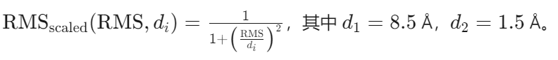
必填参数,用于DockQ计算的Native复合物结构,PDB格式,一般为实验解析的结构。
必填参数,用于DockQ计算的Model复合物结构,PDB格式,一般为AI模型预测或者分子对接等得到的模拟结构。
可选参数,指定Native结构与Model结构中的链对应关系。相对应的链名之间用逗号分隔,多组链对应时,组间用分号分隔,如:A,E;B,D;C,F表示:
注意:
1,设置该参数时,模块将根据设置的链对应关系来计算DockQ,如不设置该参数,模块会自动匹配所有有界面接触的两条链之间的对应关系,并计算匹配到的所有两条链的DockQ。
2,在特定场景中,计算DockQ时,可能希望合并某些链作为整体来考虑。比如抗原-抗体复合物中,希望将抗体的重、轻链作为一个整体,计算与抗原之间的DockQ值。这种情况,可以在指定mapping参数时,将需要合并的链名写在一起即可,比如C,F;AB,ED 表示:
输出结果文件名称,默认为dockq_res.csv
预测结果文件dockq_res.csv,包含以下信息:
| 列名 | 说明 |
|---|---|
| Native_chains | Native结构中用于计算DockQ的链名,多个链名用分号分隔 |
| Model_chains | Model结构中用于计算DockQ的链名,多个链名用分号分隔 |
| DockQ | 计算得到的DockQ数值。DockQ的分数范围为0到1,分数越高表示模型质量越好。 |
| iRMSD | 界面上两个原子相距10 Å内的原子集合的RMSD |
| LRMSD | 将预测的复合体和真实复合体的两条链中较长的链叠合后,较短链的RMSD |
| fnat | 预测复合体在交界面上的作用残基在真实复合体中的比例 |
| fnonnat | 预测复合体在交界面上的作用残基不在真实复合体中的比例 |
| F1 | 预测复合体在交界面上的作用残基是否在真实复合体中,对应的精确率和召回率的调和平均值 |
| clashes | 预测复合体中界面残基存在clash的数量,当两个残基的距离小于2Å时视为clash |
DockQ is a tool and metric used to evaluate the quality of predicted protein-protein complex structures. It combines three related but independent quality assessment metrics—Fnat, LRMS, and iRMS—into a single score ranging from 0 to 1 to assess the accuracy of docking models. A higher DockQ score indicates better model quality. Based on the DockQ score, docking models can be classified as follows:
| Score Range | Quality Category |
|---|---|
| 0.00 ≤ DockQ < 0.23 | Incorrect |
| 0.23 ≤ DockQ < 0.49 | Acceptable quality |
| 0.49 ≤ DockQ < 0.80 | Medium quality |
| DockQ ≥ 0.80 | High quality |
DockQ is computed using the following formula:
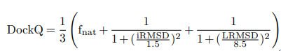
Where:
LRMSD and iRMSD are scaled using the following equations:

Required. The native (reference) structure in PDB format used for DockQ calculation, typically derived from experimental data.
Required. The model structure in PDB format to be evaluated by DockQ, typically generated by AI models or docking simulations.
Optional. Specifies the chain correspondence between the native and model structures. Chain names are separated by commas for each pair, and semicolons are used to separate multiple pairs.
For example: A,E;B,D;C,F means:
Note:
When this parameter is provided, the module uses the specified mapping for DockQ calculation.
If not set, the module will automatically match all chain pairs with interface contacts and calculate DockQ for each matched pair.
In specific scenarios, it may be necessary to consider merged chains as a single unit (e.g., heavy and light chains of an antibody). For such cases, multiple chains can be combined in the mapping, e.g., C,F;AB,ED means:
Output file name for DockQ results. The default is dockq_res.csv.
The result file dockq_res.csv contains the following information:
| Column Name | Description |
|---|---|
| Native_chains | Chains in the native structure used for DockQ calculation (separated by semicolons) |
| Model_chains | Chains in the model structure used for DockQ calculation (separated by semicolons) |
| DockQ | Computed DockQ score. The DockQ score ranges from 0 to 1, with higher scores indicating better model quality. |
| iRMSD | Interface RMSD of atoms within 10 Å |
| LRMSD | RMSD of the shorter chain after aligning the longer chains |
| fnat | Fraction of native interface contacts |
| fnonnat | Fraction of non-native interface contacts |
| F1 | F1-score combining precision and recall for predicted interface residues |
| clashes | Number of clashes (residue pairs < 2 Å apart) in the predicted complex |
Mirabello C, Wallner B. DockQ v2: improved automatic quality measure for protein multimers, nucleic acids, and small molecules. Bioinformatics. 2024 Oct 1;40(10):btae586; DOI: 10.1101/2024.05.28.596225
基于PPI-Graphomer模型预测蛋白-蛋白结合亲和力,该模型是一种专门感知界面残基作用的Graph Transformer模型,同时结合了多模态预训练模型,效果显著优于已有主流方法。
模型设计采用:序列 + 结构 + 图神经网络三合一
步骤一:特征提取,蛋白语言模型 + 结构模型协同
步骤二:核心模块,PPI-Graphomer(界面建模利器)
借鉴微软提出的 Graphormer 思想,引入结构感知的图 Transformer 模块,具体包括:
| 编码方式 | 描述 |
|---|---|
| 氨基酸对类型编码 AAType(vᵢ,vⱼ) | 区分不同氨基酸组合,推测物理作用趋势 |
| 相互作用力编码 Interact(vᵢ,vⱼ) | 捕捉氢键、盐桥、π堆叠等相互作用数量 |
| 距离权重 Dij + 接口遮罩 | 仅关注跨链、7Å内的残基对,提高关注焦点准确性 |
这些信息被作为注意力偏置项加入到 Transformer 的 Attention 计算中,强化模型对关键界面信息的关注,最终获得接口表征。
步骤三:特征拼接 + 回归预测
使用“跳跃连接式”结构(skip-connection),将界面信息与全局序列结构信息拼接后输入 MLP 预测亲和力(ΔG),输出结果用于与真实值比较回归损失。
模型整体架构示意图如下:
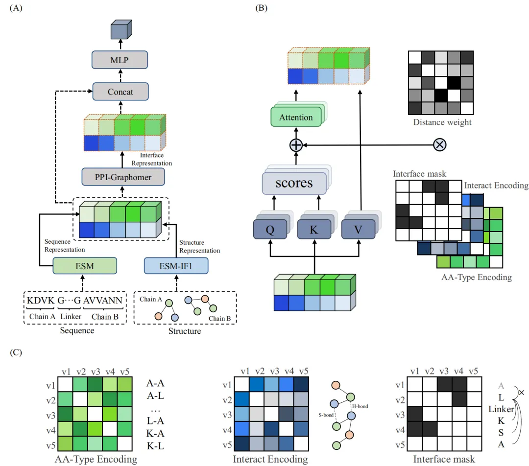
数据集与训练配置如下:
主训练集:PDBbind(共 2376 条蛋白复合物,均转化为ΔG);
测试集:
Affinity Benchmark v1(Test set 1,75 个样本)
PDBbind 精炼子集(Test set 2,87 个样本)
预处理:
移除序列过长(>2000 残基)样本;
使用 BLAST 排除训练集中与测试集相似度>65%的样本,防止数据泄露;
模型参数:
Graphomer 层数:2 层;
Attention 头数:8;
训练轮次:20 epoch;
使用 A40 GPU,推理内存仅需 4GB。
模型预测效果如下:

与其他方法的结果比较如下:
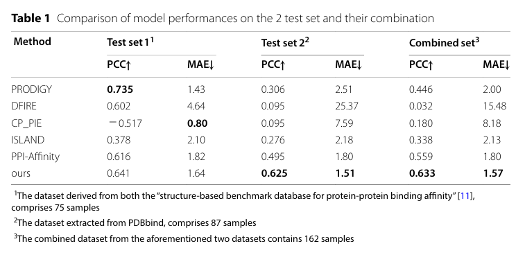
蛋白复合物结构,格式支持 .pdb 或 .cif。蛋白长度需小于2000AA(超过时会略过)。
蛋白复合物结构,支持多个复合物结构打包进行批量预测,格式支持 .tar、.tar.*z 或 .zip,最大支持1000个结构。
亲和力预测的结果文件名,默认为PPI_pred.csv
亲和力预测结果文件PPI_pred.csv,包含以下信息:
| 列名 | 说明 |
|---|---|
| Name | 结构名称 |
| Binding_Affinity (kcal/mol) | 预测的亲和力,为Gibbs自由能,单位为kcal/mol。负得越多,亲和力越强。注意:所提供的能量是复合物中所有链之间的亲和力总和。 |
This module predicts protein–protein binding affinity. It is powered by the PPI-Graphomer model, a graph transformer architecture specifically designed to capture interface residue interactions. The model integrates multimodal pretrained features and significantly outperforms existing mainstream approaches.
The model design integrates sequence + structure + graph neural network in a unified framework.
Step 1: Feature Extraction – Coordinated Protein Language and Structure Modeling
Step 2: Core Module – PPI-Graphomer (Interface Modeling Engine)
Inspired by Microsoft’s Graphormer, a structure-aware graph transformer module is introduced. It includes:
| Encoding Type | Description |
|---|---|
Amino Acid Pair Encoding AAType(vᵢ,vⱼ) |
Differentiates amino acid combinations to infer physical interaction trends |
Interaction Force Encoding Interact(vᵢ,vⱼ) |
Captures number of interactions such as hydrogen bonds, salt bridges, and π-stacking |
Distance Weight Dij + Interface Mask |
Focuses only on inter-chain residue pairs within 7Å to enhance attention accuracy |
These encodings are used as attention biases in the transformer’s attention mechanism, reinforcing the model’s focus on key interfacial residues to derive meaningful interface representations.
Step 3: Feature Fusion + Affinity Regression
Using a skip-connection design, the interface features are concatenated with global sequence and structure features and input into an MLP to predict binding affinity (ΔG). The predicted values are compared with ground truth to compute regression loss.
The overall model architecture is illustrated below:

Primary training dataset: PDBbind (2,376 protein complexes, all converted to ΔG);
Test datasets:
Preprocessing:
Model Hyperparameters:
Prediction Performance:
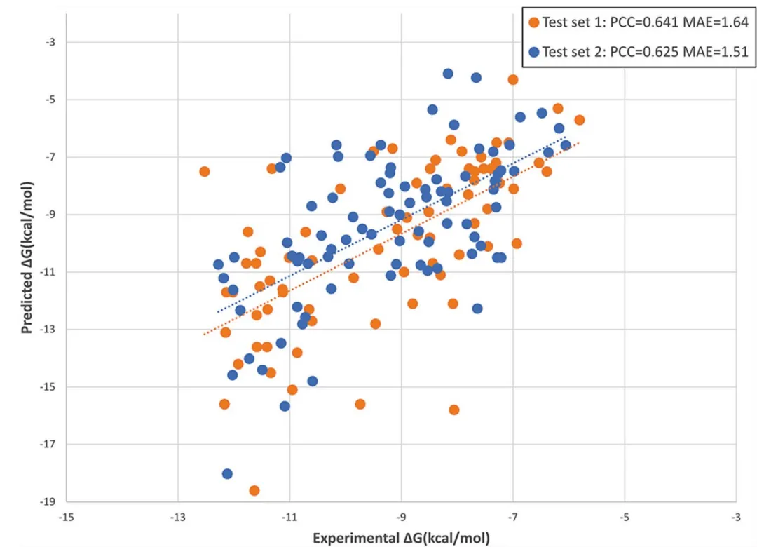
Comparison with Other Methods:

Protein-complex structure; accepted formats: .pdb or .cif.
The protein must be shorter than 2,000 amino acids (structures exceeding this limit will be skipped).
Protein-complex structures for batch prediction; submit multiple complexes packed into a single archive.
Accepted archive formats: .tar, .tar.*z, or .zip, containing up to 1,000 structures.
Filename for the prediction results. Default is PPI_pred.csv.
The output file PPI_pred.csv contains:
| Column | Description |
|---|---|
| Name | Name of the structure |
| Binding_Affinity (kcal/mol) | Predicted binding affinity (Gibbs free energy) in kcal/mol.The more negative the value, the stronger the affinity. Note: The provided energy represents the total affinity among all chains within the complex. |

该模块计算蛋白质表面静电和疏水作用相对富集的区域,用于显示出在蛋白质-蛋白质相互作用中其重要作用的区域,这对于预测基于非共价弱相互作用的可逆的聚集现象尤其有用。尤其是,疏水相互作用长期被认为是大分子间吸引相互作用的主要组成部分。对于抗体,静电相互作用牵涉到了自聚集,而偶极-偶极相互作用被认为是导致β-折叠的纤维化的原因。同时,也可以通过WeView界面对蛋白结构进行Patch分析。
v2.1 更新内容
蛋白的结构文件,PDB格式
pH值,用于蛋白质子化判断
抗体编号方法,其中 no_use 不使用编号
Hydrophobic cutoff是一个以疏水性氨基酸(通常包括Leu,Ile,Val,Phe,Trp和Met)为基础定义的截断值,用于将表面上疏水性氨基酸的数量与表面面积相比较,从而筛选出可能具有重要生物学功能的区域。一般来说,Patch区域中获得的化学性质信息会根据其表面密度和具有高疏水性氨基酸的数量而有所变化。
Positive Cutoff是一个以阳离子氨基酸为基础定义的截断值,用于将表面上阳离子氨基酸的数量与表面面积相比较,从而筛选出可能具有重要生物学功能的区域。一般来说,positive cutoff方式用于筛选出可能参与离子相互作用的蛋白质表面区域。
Negative Cutoff是一个以阴离子氨基酸为基础定义的截断值,用于将表面上阴离子氨基酸的数量与表面面积相比较,从而筛选出可能具有重要生物学功能的区域。一般来说,negative cutoff方式用于筛选出可能参与离子相互作用的蛋白质表面区域。
SASA Cutoff是一个以溶剂可及表面积为基础定义的截断值,低于截断值的patch残基会被过滤掉。是残基侧链暴露程度的百分比,相对值,范围在0-100之间。
Distance Cutoff是原子距离截断值,低于截断值的才会认为属于同一聚集块。值越小,聚集块patch越小。
Min Distance Cutoff是patch之间的距离截断值,距离小于截断值的归为同一个patch。
输出文件格式,csv或者json
通俗地讲,cutoff代表静电势能或疏水势能的强度阈值,单位是kcal/mol,超过阈值才会被计入面积。阈值越小,则patch越多。
不添加缺失原子(包括氢原子)和结构优化。
使得N-氮端的蛋白残基中性化。
使得C-氮端的蛋白残基中性化。
输出结果包括:
| 输出文件名称 | 说明 |
|---|---|
| patch_list.csv | Patch结果的csv文件。主要关注Area(Å^2)数值,代表patch的大小,越大则越可疑,重点关注100 Å以上的patch。 |
| input_prot.pdb | 质子化后的pdb结构。 |
| patch_list_sum.csv | 统计了三种patch类型(Hyd:疏水中心,Neg:负电中心,Pos:正电中心)在蛋白表面所占面积,重点关注100 Å以上的patch。 |
其中patch_list.csv,包含信息如下:
| 字段名称 | 说明 |
|---|---|
| Type | Patch的类型,Hyd:疏水中心,Neg:负电中心,Pos:正电中心 |
| Area(Å^2) | 每个Patch的蛋白质表面区域面积 |
| Residues | 每个Patch的对应的残基 |
其中patch_list_sum.csv,包含信息如下:
| 字段名称 | 说明 |
|---|---|
| Type | Patch的类型,Hyd:疏水中心,Neg:负电中心,Pos:正电中心 |
| Total Areas | Patch的蛋白质表面区域总面积 |
| Areas of The Largest | Patch的蛋白质表面区域最大面积 |
| Number of Areas More Than 100 | 超过100 Å以上的patch的数目 |
Protein Patches calculates both electrostatic (excess charge) and hydrophobic surface patches to show regions of significance with respect to protein-protein interactions. This can be particularly useful in the prediction of reversible aggregation, which typically arises from relatively weak non-covalent interactions. In particular, hydrophobic interactions have long been recognized as major contributors in high affinity interactions between macromolecules. In antibodies, electrostatic interactions have been implicated in forming self-associated aggregates [Karshikoff 2006], while dipole-dipole interactions are believed to be the cause of fibrillogenic association of β-sheets. At the same time, protein structures can also be analyzed for patches through the WeView interface.
Electrostatic patches.
The surface electrostatic field is estimated using an exponentially decaying Debye-Hückel field with a screening length of λD=3.5Å.
The map thus obtained is one mostly of excess charge close to the molecular surface.
Significant patches are established by cutting the surface along isocontour lines of absolute field value equal to 40 kcal/mol/C, keeping regions above. Finally, a default minimal patch area of 40Å2 filters out smaller, presumably less relevant, patches.
Hydrophobicity map.
The hydrophobic potential is calculated from the Wildman and Crippen octanol-water partition coefficients f=log P [Wildman 1999]:
where fi is the coefficient of atom i and g(ri) is a Fermi-type distance-dependent weighting function proposed by Heiden et al. [Heiden 1993]:
with rcut=5Å and α=1.5.
Similarly to electrostatic (excess charge) patches, significant hydrophobic patches are established by cutting the surface along isocontour lines, retaining only the portion above a potential threshold value of 0.09 kcal/mol, and filtering for a minimal patch area of 50Å2.
v2.1 updates
Protein structure file in PDB format.
pH value for protein protonation
Antibody Numbering type, no_use indicates no antibody numbering applied.
Hydrophobic Cutoff defined based on hydrophobic amino acids (usually including Leu, Ile, Val, Phe, Trp, and Met) is used to compare the number of hydrophobic amino acids on a surface with the surface area, so as to screen out areas that may have important biological functions. Generally speaking, the chemical property information obtained in the Patch region will vary according to its surface density and the number of highly hydrophobic amino acids.
Positive Cutoff is a cut-off value defined based on cationic amino acids, which is used to compare the number of cationic amino acids on the surface with the surface area to screen out areas that may have important biological functions. Generally speaking, the positive cutoff method is used to screen protein surface regions that may be involved in ion interactions.
Negative Cutoff is a value defined based on anionic amino acids, which is used to compare the number of anionic amino acids on a surface with the surface area, to screen out areas that may have important biological functions. Generally speaking, the negative cutoff method is used to screen the surface regions of proteins that may participate in ion interactions.
SASA Cutoff is a cutoff value defined on the basis of polar surface area, which is used to screen the surface regions of proteins that have enough polar surface areas.
Distance Cutoff is a cutoff value defined on the basis of neighbor atoms, which is used to adjust the size of patches. Lower values result in smaller patches.
Min Distance Cutoff is the cutoff value for neighbor patch point distance (Å). Patches with distances lower than the cutoff value would be merged.
output file format, json or csv
Do no atom addition and optimization.
The output includes:
| Output File Name | Description |
|---|---|
| patch_list.csv | A CSV file containing patch results. The main focus is on the Area (Å^2) value, which represents the size of the patch. Larger patches are considered more suspicious, with particular attention to patches larger than 100 Å. |
| input_prot.pdb | The protonated PDB structure. |
| patch_list_sum.csv | Summarizes the surface area occupied by three types of patches (Hyd: hydrophobic center, Neg: negative charge center, Pos: positive charge center) on the protein surface. Focus is placed on patches larger than 100 Å. |
Details of patch_list.csv:
The file contains the following information:
| Field Name | Description |
|---|---|
| Type | The type of patch: Hyd (hydrophobic center), Neg (negative charge center), Pos (positive charge center). |
| Area (Å^2) | The surface area of each patch on the protein. |
| Residues | The residues corresponding to each patch. |
Details of patch_list_sum.csv:
The file contains the following information:
| Field Name | Description |
|---|---|
| Type | The type of patch: Hyd (hydrophobic center), Neg (negative charge center), Pos (positive charge center). |
| Total Areas | The total surface area of patches on the protein. |
| Areas of The Largest | The largest surface area of a patch on the protein. |
| Number of Areas More Than 100 | The number of patches with an area larger than 100 Å. |
WeADApt (Wecomput ADA prediction) 是唯信开发的基于多模融合深度学习架构的免疫原性预测系统(也被熟知为AlphaMHC)。

该方法采用全新的多模融合深度神经网络架构,整合了近10亿条与免疫原性相关的湿实验数据(包括亲和力数据、呈递数据、NGS数据、质谱数据等)进行训练,有机地将多个与免疫原性相关的模型融合,构成一个高效的免疫反应模拟系统,可准确地模拟蛋白、抗体、多肽、疫苗等生物药的免疫原性,并能鉴别潜在的免疫原性的T细胞表位(引起临床人体免疫应答的肽段),实现了从序列到临床免疫原性风险的端到端的预测,并通过了数百条来自FDA、EMA的临床真实免疫原性数据(包括单/多特异性抗体和重组蛋白等)的验证测试。
该版本相比v4.1进一步提升了预测的特异性,且对不同风险水平的表位的区分度更高,结果对于去免疫原性改造更有指导性。
V4.2版本相对于上个版本v4.1主要有以下改进:
我们从FDA和EMA的临床试验中收集了200余个已知免疫原性的分子及其ADA的分布,计算模型预测值与真实ADA发生率的相关性,以测试预测性能。
在二分类测试中,将>20% ADA定义为高风险,20%以下定义为低风险。

使用唯信收集整理的166个临床及上市单抗的ADA数据的测试结果如下图所示,0.2分作为单抗的高/低风险的阈值,WeADApt表现出了最好的分类能力,准确率为86%,召回率为88%,富集率(AUC)为0.87,超过了行业知名学术软件IEDB、NetMHCllpan等。
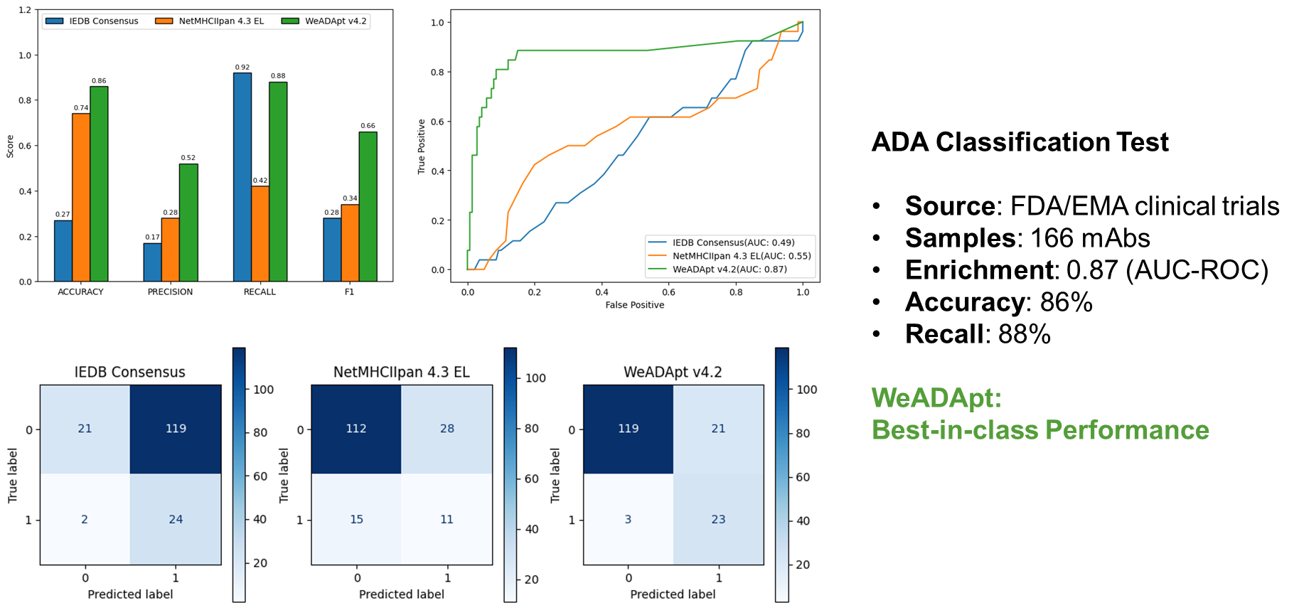
在EpiVax论文中公开的42个临床抗体分子的数据集上,WeADApt的预测结果与ADA的相关性超过了知名的商业软件EpiMatrix(R^2=0.52 vs R^2=0.42)。
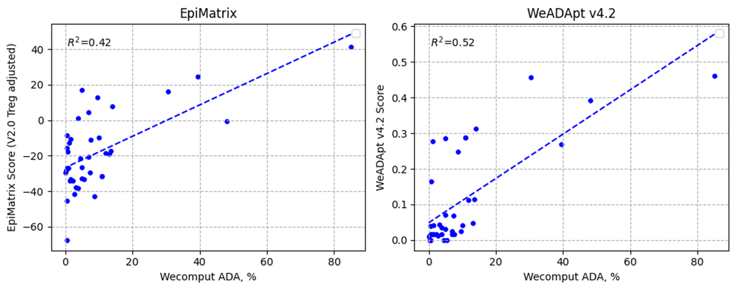
WeADApt被设计为兼容各类的分子形式,不论是对称还是非对称、是否有重复结构域的任意蛋白分子,仅需输入不重复的链即可(重复链全部输入也会自动处理)。
对比下图,WeADApt对于双抗的预测分数会相比实际ADA较单抗偏高,因此高风险的阈值建议比单抗相应提高至0.4附近。
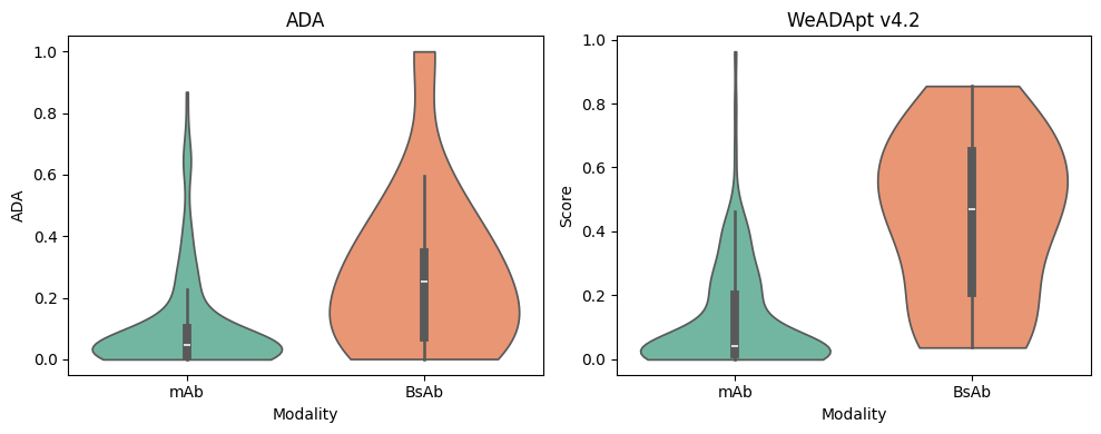
本系统仅从序列水平预测产生的影响,因此尤其适合同类靶点和相同MOA分子的相对比较和筛选。
新项目可以优先使用v4.2。对于已经使用过v4.1的项目,如果发现结果差异较大,可以参照已知临床分子的结果(比如阳性对照等),以一致性更高的版本为准。在可接受的情况下,尽量切换到v4.2。
实际项目中对于高风险阈值的定义,除了按照程序默认的单双抗0.2/0.4的标准之外,也可以以项目的阳性分子作为基准,因为不同靶点或MOA对于绝对值的影响还是蛮大的。
WeAdapt 4.2 计费规则
WeAdapt 4.2 采用阶梯式动态计费机制,根据提交的序列数量分段计费,具体规则如下:
WeADApt (Wecomput Anti-Drug Antibody prediction), internally codenamed AlphaMHC, is Wecomput’s next-generation immunogenicity predictor built on a multimodal deep-learning framework.
The platform employs a novel multimodal deep neural network trained on nearly one billion wet-lab records spanning affinity assays, antigen-presentation data, NGS profiles and mass-spectrometry spectra. By fusing orthogonal immunogenic signals, the model functions as a high-throughput in-silico immune-response simulator that accurately forecasts the immunogenic potential of biologics—including proteins, antibodies, peptides and vaccines—and pinpoints clinically relevant T-cell epitopes. The pipeline delivers end-to-end risk prediction directly from sequence and has been validated against hundreds of human immunogenicity datapoints curated by the FDA and EMA, covering both mono- and multi-specific antibodies as well as recombinant proteins.
Relative to v4.1, v4.2 delivers markedly higher specificity and sharper resolution between epitopes of differing risk levels, providing clearer guidance for de-immunization campaigns.
Key improvements over v4.1
We compiled >200 molecules with known clinical immunogenicity profiles and their observed ADA incidence from FDA- and EMA-led trials, then quantified the correlation between predicted and actual ADA rates. In binary classification, an ADA incidence >20 % was defined as high-risk and ≤20 % as low-risk.
Using a Wecomput-curated dataset of 166 clinically tested or marketed mAbs, we set a high-/low-risk threshold of 0.20. WeADApt achieved 86 % accuracy, 88 % recall and an AUC of 0.87—outperforming widely used academic tools such as IEDB and NetMHCIIpan.
On the dataset of 42 clinical antibody molecules published by EpiVax, the ADA prediction results of WeADApt showed a stronger correlation with observed ADA outcomes than the well-known commercial software EpiMatrix.
WeADApt is designed to be compatible with a wide range of molecular formats, regardless of whether the protein is symmetric or asymmetric, or contains repeated domains. Users only need to input the non-redundant chains (repeated chains will be automatically processed if included).
As shown in the figure below, WeADApt tends to yield slightly higher prediction scores for bispecific antibodies compared to monoclonal antibodies with similar observed ADA outcomes. Therefore, it is recommended to adjust the high-risk threshold upward to around 0.4 for bispecific molecules.
New projects are recommended to use version 4.2 by default.
For ongoing projects that have already used version 4.1, if significant differences in results are observed, users may refer to known clinical molecules (e.g., positive controls) and adopt the version that shows higher consistency.
Where feasible, switching to version 4.2 is encouraged.
In certain projects, the definition of high -risk thresholds can go beyond the default cutoffs (0.20 for mAbs, ~0.40 for BsAbs), project-specific positive controls can be used to calibrate thresholds, as target biology and MOA heavily influence absolute risk scores.
该模块结合界面接触特征与非相互作用表面(NIS)特征,用于预测蛋白-蛋白结合亲和力,并可输出接触界面的残基信息。模块基于PRODIGY模型,该模型通过线性回归利用界面接触点和NIS的物理化学性质来估算结合亲和力,这些性质已被验证对亲和力具有显著影响。
以下为亲和力的计算公式:

公式中的 ICsxxx/yyy 表示在相互作用的两个蛋白之间检测到的界面接触点数,xxx/yyy表示接触残基的类型(带电/极性/非极性等),例如 ICscharged/apolar 表示带电残基与非极性残基之间的接触点数量。若两个残基之间任意重原子的距离小于5.5 Å,则视为发生了接触。
该模型在81个复合物的数据集上进行了验证,预测亲和力与实验值之间的皮尔逊相关系数为0.73(p < 0.0001),均方根误差(RMSE)为1.89 kcal/mol。

蛋白复合物的结构文件,格式支持 .pdb 或 .cif。支持多个复合物结构打包进行批量预测,压缩格式支持 .tar、.tar.gz 或 .zip。注意:支持最大结构文件数量为1000
用于将结构中的多个链组合为组,组内链作为整体,仅计算组与组之间的结合亲和力。组合格式为:组内链名用逗号分隔,组与组之间用分号分隔。
示例:H,L;A 表示将链 H 和 L 作为一组,链 A 作为另一组,计算这两组之间的亲和力。
注意:
输出链间接触界面的残基对信息。
预测结果文件名,默认值为 prodigy_output.csv。
接触界面残基对的结果文件名,默认值为 contacts.txt。
预测结果文件 prodigy_output.csv 包含以下信息:
| 列名 | 说明 |
|---|---|
| Name | 结构名称 |
| Binding_Affinity (kcal/mol) | 预测的结合亲和力,单位为 kcal/mol,值越小越好,负得越多表示结合越强 |
| Dissociation_Constant (25.0˚C) | 根据公式 ΔG = RTlnKd 计算出的25°C下的解离常数 |
| Intermolecular Contacts | 接触残基对总数 |
| Charged_Charged Contacts | 带电残基-带电残基的接触对数 |
| Charged_Polar Contacts | 带电残基-极性残基的接触对数 |
| Charged_Apolar Contacts | 带电残基-非极性残基的接触对数 |
| Polar_Polar Contacts | 极性残基-极性残基的接触对数 |
| Apolar_Polar Contacts | 非极性残基-极性残基的接触对数 |
| Apolar_Apolar Contacts | 非极性残基-非极性残基的接触对数 |
| Percentage of Apolar NIS | 非极性非相互作用表面的百分比 |
| Percentage of Charged NIS | 带电非相互作用表面的百分比 |
可选接触界面结果文件 Contacts.txt,每行记录一个接触残基对,包含残基名称、编号及所在链名。
若启用批量模式,在设置contacts参数后,将给出打包文件:
contacts.tar.gz:接触残基对结果This module predicts protein-protein binding affinity by combining interfacial contact features with non-interacting surface characteristics. It also provides residue-level information for the contact interface. The module is based on the PRODIGY model, which applies linear regression using properties of interfacial contacts and non-interacting surfaces (NIS), both of which have been shown to influence binding affinity.
The binding affinity is calculated using the following formula:

ICsxxx/yyy represent the number of interfacial contact points found between interacting protein 1 and interacting protein 2, categorized by the polarity/charge of the interacting residues (e.g., ICscharged/apolar indicates the number of interfacial contact points between charged and apolar residues). Two residues are considered to be in contact if any of their heavy atoms are within 5.5 Å of each other.
The model’s prediction accuracy was evaluated using a dataset of 81 complexes. The Pearson correlation coefficient between predicted and experimental binding affinities is 0.73 (p < 0.0001), with a root-mean-square error (RMSE) of 1.89 kcal/mol⁻¹.
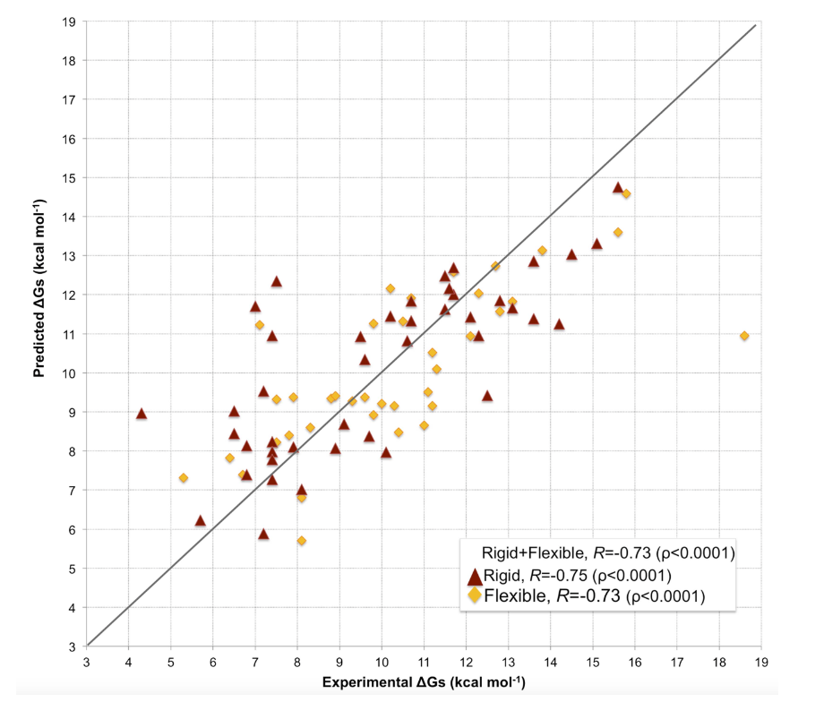
The protein complex structure in PDB or CIF format. Multiple complex structures can be packaged together for batch prediction. Supported package formats: .tar, .tar.gz, or .zip. The supported maximum number of structures is 1000.
Allows grouping of multiple chains in the structure. Chains in the same group are treated as a single unit, and binding affinity is only calculated between groups. Use chain IDs to define groups: separate chains in the same group with commas, and separate groups with semicolon.
Example: H,L;A means chains H and L are treated as one group, and chain A as another group. The binding affinity is then calculated between these two groups.
Note:
Outputs residue pairs at the inter-chain contact interface.
Filename for the binding affinity prediction result. Default: prodigy_output.csv
Filename for the contact interface residue pairs. Default: contacts.txt
The binding affinity prediction result is saved in prodigy_output.csv, which includes the following columns:
| Column Name | Description |
|---|---|
| Name | Structure name |
| Binding_Affinity (kcal/mol) | Predicted binding affinity in kcal/mol. The smaller the value, the better. The more negative it is, the stronger the binding. |
| Dissociation_Constant (25.0˚C) | Dissociation constant at 25°C, calculated using: ΔG = RTlnKd |
| Intermolecular Contacts | Total number of interfacial residue pairs |
| Charged_Charged Contacts | Number of contacts between charged residues |
| Charged_Polar Contacts | Number of contacts between charged and polar residues |
| Charged_Apolar Contacts | Number of contacts between charged and apolar residues |
| Polar_Polar Contacts | Number of contacts between polar residues |
| Apolar_Polar Contacts | Number of contacts between apolar and polar residues |
| Apolar_Apolar Contacts | Number of contacts between apolar residues |
| Percentage of Apolar NIS | Percentage of apolar non-interacting surface |
| Percentage of Charged NIS | Percentage of charged non-interacting surface |
The optional contact interface file Contacts.txt lists one contacting residue pair per line, including residue names, numbers, and chain IDs.
In batch mode:
contacts.tar.gz该模块是抗体人源化设计流程中分组模块,根据Mutation Score模块输出的回复突变评分表对回复突变进行分组,并返回突变后的序列。
更新内容:
抗体CDR区嫁接后序列文件,FASTA格式,由Grafting模块生成
抗体序列文件,FASTA格式
人源化突变评分文件,CSV格式,由Mutation Score模块生成
指定输出的突变序列文件名称,FASTA格式
打分分组的截断值,逗号分割,例如:2,5,10表示将氨基酸突变评分大于10的为一组,5~10的氨基酸为一组,小于2的氨基酸分为一组。
指定输出的回复突变的文件
普通抗体Antibody或者纳米抗体Nanobody
突变组合的截断值,Mutation Score模块中输出的氨基酸回复突变打分大于截断值的氨基酸参与生成突变组合
高于截断值的突变自动进行回复突变
每条链回复突变打分在Combination Min Cutoff与Combination Max Cutoff之间的选择打分前n个位置进行组合突变
根据不同截断值得到突变分组结果文件mutate_policy.json。
根据组合突变截断值得到的突变分组结果文件combination_mutate_policy.json,高通量人源化设计流程。
Back mutation grouping in the antibody humanization, which groups the back mutations based on the mutation scoring table generated by the Mutation Score module.
Sequence file of the antibody CDR region after grafting, in FASTA format, generated by the Grafting module.
Sequence file of the antibody, in FASTA format.
Humanization mutation score file, in CSV format, generated by the Mutation Score module.
Specify the name of the output mutation sequence file, in FASTA format.
Cutoff values for scoring grouping, separated by commas. For example, 2,5,10 indicates grouping amino acid mutations with scores greater than 10 in one group, amino acids with scores between 5 and 10 in another group, and amino acids with scores less than 2 in a separate group.
Specify the file for the output of back mutations.
Antibody or Nanobody
Cutoff value for mutation combinations. Amino acids with scores (generated from Mutation Score module) greater than the cutoff value are involved in the mutation combinations.
Mutations above the cutoff value automatically undergo reversion mutations.
For each chain, select the top n positions with back mutation scores between the Combination Min Cutoff and the Combination Max Cutoff for combination mutations.
The mutation grouping results file mutate_policy.json is generated based on different cutoff values.
The mutation grouping results file combination_mutate_policy.json is generated based on combination cutoff values.
该模块具有两方面的功能:
1,用于预测肽段(长度不超过10个氨基酸)被18种基质金属蛋白酶(MMPs)切割的效率。
2,基于指定的目标切割谱(如:仅被MMP13切割),生成相应的多肽底物。
模块基于CleaveNet模型实现,CleaveNet是一种基于深度学习的蛋白酶底物设计工具,通过整合预测与生成技术,实现了从“虚拟筛选”到“智能设计”的转变。
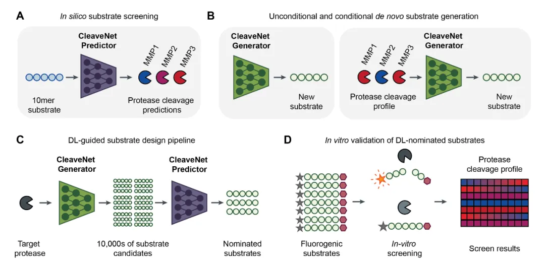
CleaveNet包含两个核心模块:
预测模块
生成模块
这一端到端的设计流程显著提高了底物设计的效率和精准性,为蛋白酶研究提供了一种全新的计算驱动方法。
实验验证
为评估CleaveNet的实际应用能力,研究团队以MMP13(一种与癌症转移、伤口愈合和骨关节炎相关的胶原酶)为目标,设计并合成了95条肽段底物,并通过荧光共振能量转移(FRET)技术验证其切割效率。实验结果表明:
这些结果验证了CleaveNet在设计高效且特异性底物方面的能力,同时也展示了其揭示未知底物偏好的潜力。
必填参数,多肽序列,txt或fasta格式,支持多条(txt格式时,每行放置一条多肽,最多支持1000条多肽)。注意:多肽长度不能超过10个残基,超过长度的多肽序列会自动被过滤掉。
txt格式实例如下:
LRVFL
FMPLNFTASG
LGPYAMTSRG
AARFKKFATE
可选参数,预测得到的MMPs酶切概率结果文件名称,默认为“pred_cleavage.csv”。
可选参数,指定需要生成的多肽数量,默认为50。
可选参数,指定多肽生成的酶切条件,CSV文件格式。包含每种MMP酶的酶切概率Z-score值,值越大表示酶切的可能性越高,值可为负,一般阈值为2.5,大于该阈值时,表示极大可能被酶切。模型会根据设置的各种MMPs酶的酶切概率Z-score值进行多肽生成。注意:18种MMPs的Z-score数值都必须设定,不能缺少任意一种。
文件内容实例如下:
MMP1,MMP10,MMP11,MMP12,MMP13,MMP14,MMP15,MMP16,MMP17,MMP19,MMP2,MMP20,MMP24,MMP25,MMP3,MMP7,MMP8,MMP9
2.0,1.2,2.2,2.9,3.3,4.1,2.2,3.1,2.2,1.91,3.6,2.83,2.7,0.2,1.8,2.1,0.61,4.2
以上内容为一组条件,也支持多组条件同时输入,每行一组条件即可。每组条件都会生成指定数量的多肽。多组条件示例如下:
MMP1,MMP10,MMP11,MMP12,MMP13,MMP14,MMP15,MMP16,MMP17,MMP19,MMP2,MMP20,MMP24,MMP25,MMP3,MMP7,MMP8,MMP9
2.0,1.2,2.2,2.9,3.3,4.1,2.2,3.1,2.2,1.91,3.6,2.83,2.7,0.2,1.8,2.1,0.61,4.2
3.33,2.5,3.6,2.7,2.9,5.2,3.4,4.2,2.7,2.0,3.5,2.6,4.0,3.1,3.5,0.61,2.1,2.9
可选参数,指定生成的温度条件,用于控制生成多肽序列的多样性,默认为1.0,越大表示多样性越高。如果希望多样性低一些,推荐0.7,如果希望多样性再高一些,推荐1.2~1.5。
可选参数,指定序列输出文件名称,fasta或txt格式,默认为“gen_seqs.fasta”。
预测得到的MMPs酶切概率结果文件,默认为pred_cleavage.csv。包含如下内容:
| 字段名称 | 说明 |
|---|---|
| SEQ | 多肽序列 |
| MMP1,MMP2,MMP3,… | 各种MMPs蛋白酶对多肽酶切能力强弱的Z-score数值,数值越大表示酶切的可能性越高,目前的阈值为2.5,大于该阈值时,表示极大可能被酶切。 |
生成的序列文件,默认为“gen_seqs.fasta”。
This module has two functions:
Predicting the cleavage efficiency of peptides (≤10 amino acids) by 18 matrix metalloproteinases (MMPs).
Generating corresponding peptide substrates based on a specified cleavage profile (e.g., only cleaved by MMP13).
Built on the CleaveNet model, a deep - learning - based protease substrate design tool, it integrates prediction and generation, shifting from “virtual screening” to “intelligent design”.
CleaveNet has two core modules:
Prediction Module
Trained on a large - scale mRNA - displayed peptide library using a Transformer architecture.
Predicts peptide cleavage efficiency by 18 MMPs, with a test - set Pearson correlation of 0.80, outperforming traditional binary - classification models.
Reproduces known cleavage motifs and reveals new substrate preferences (e.g., methionine at P4), enhancing understanding of protease specificity.
Generation Module
Uses conditional generation. Users can set target cleavage profiles (e.g., “high MMP13 activity, low other MMP activities”) via conditional tags.
Adjusts generation direction with attention mechanisms. Generated 6 - mer peptides have 89% novelty, surpassing training data limits.
Is about 5.5 times more efficient than traditional virtual screening, supporting complex designs like “dual - protease logic gate” substrates.
This end - to - end design process improves substrate design efficiency and accuracy, offering a new computation - driven method for protease research.
Experimental Validation
To assess CleaveNet’s practicality, the team targeted MMP13 (a collagenase linked to cancer metastasis, wound healing, and osteoarthritis). They designed and synthesized 95 peptide substrates, validating cleavage efficiency via fluorescence resonance energy transfer (FRET). Results showed:
All CleaveNet - designed MMP13 substrates were efficiently cleaved. One (DL73) had 39% higher efficiency than the best training - set substrate (p<0.01).
Three substrates (e.g., DL41) were absolutely specific to MMP13, and five (e.g., DL48) had both high activity and selectivity, addressing traditional method gaps.
Analysis of generated sequences revealed leucine preference at P2 and aspartic acid’s role at P3’, offering new insights into MMP13’s specificity mechanism.
These results confirm CleaveNet’s ability to design efficient, specific substrates and its potential to uncover unknown substrate preferences.
Required parameter, peptide sequence, in txt or fasta format, supporting multiple sequences (when in txt format, place each peptide on a separate line. Supports up to 1,000 peptides.). Note: The length of the peptide cannot exceed 10 residues.
An example in txt format is as follows:
LRVFL
FMPLNFTASG
LGPYAMTSRG
AARFKKFATE
Optional parameter, the file name of the predicted MMPs cleavage probability results, default is “pred_cleavage.csv”。
Optional parameter, specify the number of peptides to be generated, default is 50.
Optional parameter, specify the cleavage conditions for peptide generation in CSV file format. It includes the Z-score values of cleavage probabilities for each type of MMP enzyme. A higher value indicates a higher likelihood of cleavage. The value can be negative. The general threshold is 2.5. When the value is above this threshold, it indicates a very high probability of being cleaved. The model will generate peptides based on the set Z-score values of cleavage probabilities for various MMPs enzymes. Note: The Z-score values for all 18 types of MMPs must be set, and none can be missing.
An example of the file content is as follows:
MMP1,MMP10,MMP11,MMP12,MMP13,MMP14,MMP15,MMP16,MMP17,MMP19,MMP2,MMP20,MMP24,MMP25,MMP3,MMP7,MMP8,MMP9
2.0,1.2,2.2,2.9,3.3,4.1,2.2,3.1,2.2,1.91,3.6,2.83,2.7,0.2,1.8,2.1,0.61,4.2
The above content is a set of conditions, and multiple sets of conditions can also be input simultaneously. Just place each set of conditions on a separate line. Peptides of the specified quantity will be generated for each set of conditions. An example of multiple sets of conditions is as follows:
MMP1,MMP10,MMP11,MMP12,MMP13,MMP14,MMP15,MMP16,MMP17,MMP19,MMP2,MMP20,MMP24,MMP25,MMP3,MMP7,MMP8,MMP9
2.0,1.2,2.2,2.9,3.3,4.1,2.2,3.1,2.2,1.91,3.6,2.83,2.7,0.2,1.8,2.1,0.61,4.2
3.33,2.5,3.6,2.7,2.9,5.2,3.4,4.2,2.7,2.0,3.5,2.6,4.0,3.1,3.5,0.61,2.1,2.9
Optional parameter, specify the temperature condition for controlling the diversity of the generated peptide sequences. The default value is 1.0. A higher value indicates higher diversity. If you want lower diversity, it is recommended to use 0.7. If you want higher diversity, it is recommended to use a value between 1.2 and 1.5.
Optional parameter, specify the output file name for the sequences in fasta or txt format. The default is “gen_seqs.fasta”.
The predicted MMPs cleavage probability results file, default is pred_cleavage.csv. It contains the following content:
| Field Name | Description |
|---|---|
| SEQ | Peptide sequence |
| MMP1, MMP2, MMP3, … | Z-score values representing the strength of cleavage by various MMPs proteases. A higher value indicates a higher likelihood of cleavage. The current threshold is 2.5. If the value is above this threshold, it indicates a very high probability of being cleaved. |
The generated sequence file, default is “gen_seqs.fasta”.
该模块用于分析和可视化蛋白质表面的静电特性,这对分子识别、蛋白质溶解性、粘度和抗体的可开发性等过程至关重要。它主要通过定义“Patch”来识别和量化蛋白质表面的静电势,这些Patch是具有统一正或负电势值的连接区域。
主要功能和特点:
蛋白结构文件,PDB格式。
分子表面的类型:sas或者ses。以下是两个选项的解释:
探针半径,单位为纳米(默认:0.14)。
Patch面积(area )阈值,单位为Ų。如果 Size Cutoff = 0,则不过滤任何 patch,即所有 patch 都会被保留。
pH 值。
输出Patch文件名称
输出结果包括:
| 输出文件名称 | 说明 |
|---|---|
| patches.csv | 识别出的蛋白质表面静电Patch的信息。 |
| apbs.pqr | APBS计算静电势的输入文件。PQR文件类似于PDB文件,但包含了每个原子的电荷和半径信息。 |
| apbs.pqr.dx | 通过APBS计算得到的静电势分布数据。DX文件是网格格式,描述了蛋白质周围空间的静电势值。 |
| apbs.pdb | APBS计算静电势的PDB文件 |
其中patches.csv包括信息如下:
| 字段名称 | 说明 |
|---|---|
| nr | 代表Patch的编号。这是每个识别出的静电Patch的唯一标识符,用于区分不同的Patch。 |
| type | 表示Patch的类型,通常为“positive”或“negative”,指示Patch的电荷性质是正电还是负电。 |
| npoints | Patch中包含的表面点的数量。这些点构成了Patch在蛋白质表面上的区域。 |
| area | Patch的面积,单位为Ų。这表示Patch在蛋白质表面上覆盖的物理面积。 |
| value | Patch的总静电势值,通常为Patch内所有点的静电势值的总和或平均值。这反映了Patch的整体静电强度。 |
| residue | Patch中的氨基酸残基,通常是Patch所在区域的一个代表性残基。这个残基可能是Patch中电荷最集中的位置或最显著的氨基酸。其他的氨基酸编号与apbs.pdb对应。 |
This module is designed for analyzing and visualizing the electrostatic properties of protein surfaces, which are critical for processes such as molecular recognition, protein solubility, viscosity, and antibody developability. It primarily identifies and quantifies the electrostatic potential on protein surfaces by defining “patches,” which are connected regions with uniform positive or negative potential values.
Key Features:
Electrostatic Potential Calculation:
This tool uses APBS (Adaptive Poisson-Boltzmann Solver) to compute electrostatic potentials. Additionally, it can accept user-provided potential maps or mappings based on hydrophobicity scales.
Molecular Surface Generation:
The tool generates molecular surfaces and maps the calculated electrostatic potentials onto these surfaces. The surface can then be visualized using color coding to indicate positive and negative regions.
Patch Identification:
It identifies and quantifies different positive and negative electrostatic patches on the protein surface, which are crucial for understanding protein-protein interactions and antibody development.
The protein structure file in PDB format.
The type of molecular surface: SAS or SES. Below are explanations for the two options:
The radius of the probe, measured in nanometers (default: 0.14).
Patch area threshold (area), measured in Ų. If Size Cutoff = 0, no patch will be filtered, meaning all patches will be retained.
The pH value.
The name of the output file for identified patches.
The output includes the following files:
| File Name | Description |
|---|---|
patches.csv |
Information about the identified electrostatic patches on the protein surface. |
apbs.pqr |
Input file for APBS electrostatic potential calculations. PQR files are similar to PDB files but include charge and radius information for each atom. |
apbs.pqr.dx |
Electrostatic potential distribution data calculated by APBS. DX files are grid-format files describing the electrostatic potential values in the space surrounding the protein. |
apbs.pdb |
PDB file with electrostatic potential information calculated by APBS. |
The patches.csv file includes the following information:
| Field Name | Description |
|---|---|
| nr | Patch number. This is a unique identifier for each identified electrostatic patch. |
| type | Patch type, typically “positive” or “negative,” indicating whether the patch is positively or negatively charged. |
| npoints | The number of surface points in the patch, which defines the region of the patch on the protein surface. |
| area | The area of the patch in Ų, representing the physical coverage of the patch on the protein surface. |
| value | The total electrostatic potential value of the patch, usually the sum or average of all potential values within the patch. This indicates the overall electrostatic intensity of the patch. |
| residue | Representative amino acid residue within the patch, typically the residue with the highest charge concentration or the most prominent residue in the patch. Other residue numbers correspond to the apbs.pdb file. |
该模块计算蛋白质表面静电和疏水作用相对富集的区域,用于显示出在蛋白质-蛋白质相互作用中其重要作用的区域,这对于预测基于非共价弱相互作用的可逆的聚集现象尤其有用。尤其是,疏水相互作用长期被认为是大分子间吸引相互作用的主要组成部分。对于抗体,静电相互作用牵涉到了自聚集,而偶极-偶极相互作用被认为是导致β-折叠的纤维化的原因。同时,也可以通过WeView界面对蛋白结构进行Patch分析。
V2 更新内容
蛋白的结构文件,PDB格式
Hydrophobic cutoff是一个以疏水性氨基酸(通常包括Leu,Ile,Val,Phe,Trp和Met)为基础定义的截断值,用于将表面上疏水性氨基酸的数量与表面面积相比较,从而筛选出可能具有重要生物学功能的区域。一般来说,Patch区域中获得的化学性质信息会根据其表面密度和具有高疏水性氨基酸的数量而有所变化。
Positive Cutoff是一个以阳离子氨基酸为基础定义的截断值,用于将表面上阳离子氨基酸的数量与表面面积相比较,从而筛选出可能具有重要生物学功能的区域。一般来说,positive cutoff方式用于筛选出可能参与离子相互作用的蛋白质表面区域。
Negative Cutoff是一个以阴离子氨基酸为基础定义的截断值,用于将表面上阴离子氨基酸的数量与表面面积相比较,从而筛选出可能具有重要生物学功能的区域。一般来说,negative cutoff方式用于筛选出可能参与离子相互作用的蛋白质表面区域。
SASA Cutoff是一个以溶剂可及表面积为基础定义的截断值,低于截断值的patch会被过滤掉。
Distance Cutoff是原子距离截断值,低于截断值的才会认为属于同一聚集块。值越小,聚集块patch越小。
Min Distance Cutoff是patch之间的距离截断值,距离小于截断值的归为同一个patch。
输出文件格式,csv或者json
通俗地讲,cutoff代表静电势能或疏水势能的强度阈值,单位是kcal/mol,超过阈值才会被计入面积。阈值越小,则patch越多。
不添加缺失原子(包括氢原子)和结构优化。
使得N-氮端的蛋白残基中性化。
使得C-氮端的蛋白残基中性化。
输出结果包括:
| 输出文件名称 | 说明 |
|---|---|
| patch_list.csv | Patch结果的csv文件。主要关注Area(Å^2)数值,代表patch的大小,越大则越可疑,重点关注100 Å以上的patch。 |
| input_prot.pdb | 质子化后的pdb结构。 |
| patch_list_sum.csv | 统计了三种patch类型(Hyd:疏水中心,Neg:负电中心,Pos:正电中心)在蛋白表面所占面积,重点关注100 Å以上的patch。 |
其中patch_list.csv,包含信息如下:
| 字段名称 | 说明 |
|---|---|
| Type | Patch的类型,Hyd:疏水中心,Neg:负电中心,Pos:正电中心 |
| Area(Å^2) | 每个Patch的蛋白质表面区域面积 |
| Residues | 每个Patch的对应的残基 |
其中patch_list_sum.csv,包含信息如下:
| 字段名称 | 说明 |
|---|---|
| Type | Patch的类型,Hyd:疏水中心,Neg:负电中心,Pos:正电中心 |
| Total Areas | Patch的蛋白质表面区域总面积 |
| Areas of The Largest | Patch的蛋白质表面区域最大面积 |
| Number of Areas More Than 100 | 超过100 Å以上的patch的数目 |
Protein Patches calculates both electrostatic (excess charge) and hydrophobic surface patches to show regions of significance with respect to protein-protein interactions. This can be particularly useful in the prediction of reversible aggregation, which typically arises from relatively weak non-covalent interactions. In particular, hydrophobic interactions have long been recognized as major contributors in high affinity interactions between macromolecules. In antibodies, electrostatic interactions have been implicated in forming self-associated aggregates [Karshikoff 2006], while dipole-dipole interactions are believed to be the cause of fibrillogenic association of β-sheets. At the same time, protein structures can also be analyzed for patches through the WeView interface.
Electrostatic patches.
The surface electrostatic field is estimated using an exponentially decaying Debye-Hückel field with a screening length of λD=3.5Å.
The map thus obtained is one mostly of excess charge close to the molecular surface.
Significant patches are established by cutting the surface along isocontour lines of absolute field value equal to 40 kcal/mol/C, keeping regions above. Finally, a default minimal patch area of 40Å2 filters out smaller, presumably less relevant, patches.
Hydrophobicity map.
The hydrophobic potential is calculated from the Wildman and Crippen octanol-water partition coefficients f=log P [Wildman 1999]:
where fi is the coefficient of atom i and g(ri) is a Fermi-type distance-dependent weighting function proposed by Heiden et al. [Heiden 1993]:
with rcut=5Å and α=1.5.
Similarly to electrostatic (excess charge) patches, significant hydrophobic patches are established by cutting the surface along isocontour lines, retaining only the portion above a potential threshold value of 0.09 kcal/mol, and filtering for a minimal patch area of 50Å2.
V2 updates
Protein structure file in PDB format.
Hydrophobic Cutoff defined based on hydrophobic amino acids (usually including Leu, Ile, Val, Phe, Trp, and Met) is used to compare the number of hydrophobic amino acids on a surface with the surface area, so as to screen out areas that may have important biological functions. Generally speaking, the chemical property information obtained in the Patch region will vary according to its surface density and the number of highly hydrophobic amino acids.
Positive Cutoff is a cut-off value defined based on cationic amino acids, which is used to compare the number of cationic amino acids on the surface with the surface area to screen out areas that may have important biological functions. Generally speaking, the positive cutoff method is used to screen protein surface regions that may be involved in ion interactions.
Negative Cutoff is a value defined based on anionic amino acids, which is used to compare the number of anionic amino acids on a surface with the surface area, to screen out areas that may have important biological functions. Generally speaking, the negative cutoff method is used to screen the surface regions of proteins that may participate in ion interactions.
SASA Cutoff is a cutoff value defined on the basis of polar surface area, which is used to screen the surface regions of proteins that have enough polar surface areas.
Distance Cutoff is a cutoff value defined on the basis of neighbor atoms, which is used to adjust the size of patches. Lower values result in smaller patches.
Min Distance Cutoff is the cutoff value for neighbor patch point distance (Å). Patches with distances lower than the cutoff value would be merged.
output file format, json or csv
Do no atom addition and optimization.
The output includes:
| Output File Name | Description |
|---|---|
| patch_list.csv | A CSV file containing patch results. The main focus is on the Area (Å^2) value, which represents the size of the patch. Larger patches are considered more suspicious, with particular attention to patches larger than 100 Å. |
| input_prot.pdb | The protonated PDB structure. |
| patch_list_sum.csv | Summarizes the surface area occupied by three types of patches (Hyd: hydrophobic center, Neg: negative charge center, Pos: positive charge center) on the protein surface. Focus is placed on patches larger than 100 Å. |
Details of patch_list.csv:
The file contains the following information:
| Field Name | Description |
|---|---|
| Type | The type of patch: Hyd (hydrophobic center), Neg (negative charge center), Pos (positive charge center). |
| Area (Å^2) | The surface area of each patch on the protein. |
| Residues | The residues corresponding to each patch. |
Details of patch_list_sum.csv:
The file contains the following information:
| Field Name | Description |
|---|---|
| Type | The type of patch: Hyd (hydrophobic center), Neg (negative charge center), Pos (positive charge center). |
| Total Areas | The total surface area of patches on the protein. |
| Areas of The Largest | The largest surface area of a patch on the protein. |
| Number of Areas More Than 100 | The number of patches with an area larger than 100 Å. |
该模块是一种用于分子对接模拟工具,主要用于预测分子之间的结合模式和相互作用,得到分子对接的能量和结合亲和力等信息。它还可以计算和比较多个分子之间的结合能力,用于药物分子的筛选、设计和优化。AutoDock-GPU是AutoDock4.2.6的OpenCL和Cuda加速版本,其利用可并行的LGA,从而通过在多个计算单元上并行处理配体-受体结合构象。
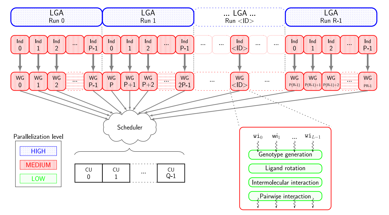
支持自行上传小分子文件(Private Ligand Library)或者选择公共分子虚筛库(Public Ligand Library)。
对接模式为刚性配体对接(rigid)或者柔性配体对接(flex),
刚性配体对接:配体自身保持刚性,经平移、旋转,在口袋内寻找合适的结合取向。
柔性配体对接:配体在固定某些非关键部位的键长、键角的前提下允许其构象发生一定程度的变化。
受体结构文件,PDB格式。要求受体原子数目不超过32768个。
配体结构文件,支持SDF、PDB、MOL格式。只会计算前100的分子。
对接口袋中心的三维坐标(XYZ),空格分割。例如:0 0 0。
对接口袋长方体盒子的大小,必须是整数,空格分割,例如 24 22 32。
每个分子保留的最大结合模式数量
虚拟筛选中保留打分排名前n个分子。
未结合状态模型选择:
保留非标准氨基酸,格式为[链名]:[残基名称]-[残基编号],如A:UNL-311。不能包含特殊离子的小分子结构。
配体结构文件,支持SDF、PDB、MOL格式。只会计算前10,000的分子。
其余参数与**Private Ligand Library (Comp<100)**模式一致。
提供17个公共分子虚筛库用于分子对接,包括:
其他参数与Private Ligand Library模式相同,公共库只允许刚性对接。
输出结果包括:
| 输出文件名称 | 说明 |
|---|---|
| TopNScores.csv | 分子对接得到的打分csv文件。输出小分子最多为10,000。 |
| complex_001.pdb | 展示配体与受体的复合物构象文件。 |
| output_ligand_topn.sdf | 筛选后配体的SDF文件。根据指定的topN数生成,最多为10,000。 |
| output_complex_topn.tar.bz2 | 小分子与受体对接后的复合物构象PDB文件压缩包,最多生成前1000小分子的复合物结构。 |
| TopNScores_Molecule_Info.csv | 当Private Ligand Library模式,该csv中不仅有打分信息,还有配体原有信息。 |
其中TopNScores.csv包括信息如下:
| 字段名称 | 说明 |
|---|---|
| Name | 对接小分子名称 |
| Bingding Energy (AutoDock GPU) | 对接打分结果,单位为kcal/mol |
| Cluster RMSD | 指一个配体构象相对于同一聚类(cluster)中的中心构象(通常是最低能量构象)的均方根偏差(RMSD)。RMSD 截断值为2.0 Å。 |
| Reference RMSD | 指对接得到的配体构象与 参考构象(通常是实验解析的晶体结构或用户指定的标准结构)之间的 RMSD。 |
其中TopNScores_Molecule_Info.csv包含TopNScores.csv的信息和SDF格式小分子原有信息。
This module is a molecular docking simulation tool primarily used for predicting molecular binding modes and interactions. It provides information on docking energy and binding affinity. Additionally, it allows for the calculation and comparison of binding abilities among multiple molecules, facilitating the screening, design, and optimization of drug molecules.
AutoDock-GPU is the OpenCL and CUDA-accelerated version of AutoDock 4.2.6, utilizing parallelizable LGA (Lamarckian Genetic Algorithm) to process ligand-receptor binding conformations in parallel across multiple computing units.

It supports private ligand file uploads (Private Ligand Library) or the selection of public virtual screening libraries (Public Ligand Library).
Docking mode can be either rigid docking or flexible docking:
100 molecules will be processed.0 0 024 22 32Defines the unbound state model:
[Chain Name]:[Residue Name]-[Residue Number], e.g., A:UNL-311.10,000 molecules will be processed.🔹 Other parameters are identical to those in Private Ligand Library (Comp <100) mode.
Provides 17 public virtual screening libraries for molecular docking, including:
🔹 Other parameters are identical to Private Ligand Library, but only rigid docking is allowed.
The docking results include:
| File Name | Description |
|---|---|
| TopNScores.csv | CSV file containing docking scores for up to 10,000 molecules. |
| complex_001.pdb | Ligand-receptor complex conformation file. |
| output_ligand_topn.sdf | Top-N selected ligands in SDF format (max 10,000). |
| output_complex_topn.tar.bz2 | Compressed file of the top 1,000 ligand-receptor complex structures in PDB format. |
| TopNScores_Molecule_Info.csv | If using the Private Ligand Library mode, this CSV includes both docking scores and original ligand information. |
📌 TopNScores.csv Fields:
| Field Name | Description |
|---|---|
| Name | Name of the docked molecule. |
| Binding Energy (AutoDock GPU) | Docking score. |
| Cluster RMSD | RMSD relative to the cluster center (default cutoff: 2.0 Å). |
| Reference RMSD | RMSD relative to the reference structure (e.g., crystal structure). |
The TopNScores_Molecule_Info.csv file contains the information from TopNScores.csv along with the original data of small molecules in SDF format.
RFantibody 是目前最先进的抗体从头生成方法,通过人工智能(AI)技术实现抗体的从头(de novo)设计,包括单域抗体(VHH)和单链抗体片段(scFv),能够精准结合用户指定的目标表位,并已通过湿实验验证其功能。
RFantibody基于蛋白质结构预测模型RoseTTAFold2(RF2)和蛋白质生成模型RFdiffusion,通过对原始RFdiffusion进行微调,开发出专用于抗体设计的RFdiffusion版本。其核心原理如下:
抗体结构特性利用:RFdiffusion在蛋白质数据库(PDB)中的抗体结构数据(约8100个抗体结构)上进行微调,重点训练抗体特有的互补决定区(CDR)loop 区域,同时保持框架结构接近用户指定的优化框架。训练过程中,通过逐步添加噪声(Cα 坐标加入三维高斯噪声,残基方向加入 SO(3) 布朗运动),网络学习预测去噪后的结构。
表位靶向设计:通过引入"热点"(Hotspot)特征,用户可指定目标蛋白上的表位,网络通过CDR loop与表位的相互作用进行设计。训练时,抗体框架以全局坐标无关的方式提供(通过二维距离和二面角矩阵表示),允许网络自由设计CDR Loop构象及抗体与目标的刚体定位。
序列设计与验证:结构设计后,使用ProteinMPNN生成CDR loop区序列,优化与目标表位的相互作用。设计的抗体通过微调后的RF2进行结构预测和自一致性验证,筛选高潜力候选分子。
支持 VHH 和 scFv 设计:RFdiffusion 不仅支持单域抗体(VHH)的设计,还可应用于单链抗体片段(scFv)的设计。scFv 设计涉及重链和轻链的所有六个 CDR 的设计。
通过上述方法,RFantibody能够生成多样化的抗体结构,显著区别于训练数据集,同时实现与目标表位的高度形状互补性和功能性结合。
RFantibody项目针对多个疾病相关表位进行了VHH和scFv设计,并通过表面等离子共振(SPR)、冷冻电镜(cryo-EM)、中和实验等手段验证了设计的有效性。以下是具体实验结果及分析:
1, 单域抗体(VHH)设计与实验验证
实验选择了多个疾病相关靶点,包括流感血凝素(HA)、呼吸道合胞病毒(RSV)位点I和III、SARS-CoV-2受体结合域(RBD)、艰难梭菌毒素B(TcdB)和IL-7Rα。以下为关键结果:
结合亲和力(KD):
中和活性(EC50):
结构准确性(cryo-EM):
亲和力成熟(OrthoRep):
2, 单链抗体片段(scFv)设计与实验验证
进一步扩展至scFv设计,涉及重链和轻链六个CDR的设计,采用结构导向的组合库策略以提高成功率。实验靶点包括TcdB的Frizzled-7表位和Phox2b/HLA-C*07:02复合物。
结合亲和力(KD):
结构准确性(cryo-EM):
3, 实验结果分析
4, 总结
RFantibody通过微调RFdiffusion网络,实现了从头设计VHH和scFv的目标,能够靶向多种疾病相关表位。实验结果显示设计的抗体具有较高的结构准确性(RMSD低至0.9 Å)和功能性(KD低至72 nM,EC50为460 nM)。cryo-EM验证了设计的原子级精度,而亲和力成熟和组合库策略进一步提升了成功率。
用于抗体设计的抗体-抗原复合物结构,PDB格式。如果指定了该参数,后续的Antigen,Antibody参数不用再指定。如果不指定该参数,则需要分别输入Antigen与Antibody的结构。
注意:当前只支持单链抗原,如存在多链时会提示错误,可以使用蛋白编辑工具去掉抗原多余的链,保留单链抗原即可。
指定抗原的结构文件,PDB格式。
说明:抗原结构通常需要截短以减少计算开销,建议保留表位周围约 10Å 的区域即可。
指定抗体的结构文件,PDB格式。
指定设计的抗体数量,默认为20。
定义需要突变设计的残基,格式为“链名称+残基编号或范围”,多段残基用逗号分隔。例如:参数设置为H27,H28,H99,H100-103,L24-32时,表示:对H链中编号为27、28、99,、100至103的残基,L链中编号为24-32的残基,进行突变设计。
注意:
1,这里的残基编号是指从1开始的残基位置顺序编号,不是原PDB文件中的残基编号。
2,如指定了该参数,则不能再指定后续的CDR参数(HCDR1-3或LCDR1-3),否则会提示参数错误。
分别指定需要设计的抗体重、轻链CDR区的长度范围。格式为:起始长度-终止长度(如:5-13),或单一长度(如:7)。
说明:这些参数定义了每个CDR区的允许长度范围,如果设置的是起始长度-终止长度(如:5-13),模型将从中均匀采样长度。如果设置的是单一长度(如:7),则该CDR将以指定长度进行设计。如果不指定某个CDR的长度范围(如:不设置H-CDR1的长度),则该CDR将保持原始结构和序列不被设计。需要指定至少一个CDR区域的长度进行设计,否则会提示错误。
对于VHH设计,仅需指定H-CDR1, H-CDR2, H-CDR3;对于scFv设计,可指定所有六个CDR。长度选择可参考自然抗体的CDR 长度分布,推荐较短的H-CDR3(如:5-13),以降低设计难度。
指定抗原上的结合位点残基,用于定义抗体结合的表位。格式为:逗号分隔的残基列表,格式为 305,456
经过抗体设计后,得到的抗体-抗原复合物结构,并根据质量评估指标进行排序。包括:
结构文件:按结构质量排序的PDB格式抗体-抗原复合物结构的打包文件 de_novo_antibody.tar及最优的设计结果rank_1.pdb
结构评分:CSV格式的评估指标表格 cdr_sequences.csv,包含如下信息:
| 字段名称 | 说明 |
|---|---|
| Design_ID | 预测结构的文件名 |
| CDR_H1/H2/H3/L1/L2/L3 | 设计后得到的CDR序列 |
| ipAE | 预测对齐误差交互值(the predicted interaction alignment error),衡量抗体与抗原结合界面的结构预测置信度,该指标反映了抗体-抗原复合物界面的结构稳定性和预测准确性,数值越小表示结合界面预测越可靠,推荐选择ipAE<10的设计进行实验验证 |
| pLDDT | 预测局部距离差异测试,衡量整体结构预测的质量和可靠性,该指标反映了抗体结构本身的稳定性和折叠质量,数值范围为 0-1.0,数值越接近1.0表示结构预测越可靠,推荐选择pLDDT > 0.8的设计进行实验验证 |
输出示例
Design_ID,CDR_H3,ipAE,pLDDT
rank_1,IAYTPGAPLF,8.91,0.92
rank_2,VAPSKTDALF,9.29,0.92
序列文件:所有设计抗体的序列汇总文件antibody_sequences.fasta
RFantibody is the most advanced de novo antibody generation method currently available. Through artificial intelligence (AI) technology, it achieves de novo design of antibodies, including single-domain antibodies (VHH) and single-chain antibody fragments (scFv), capable of precisely binding to user-specified target epitopes, with functionality validated through wet lab experiments.
RFantibody is based on the protein structure prediction model RoseTTAFold2 (RF2) and the protein generation model RFdiffusion. By fine-tuning the original RFdiffusion, a specialized version for antibody design has been developed. Its core principles are as follows:
Utilization of Antibody Structural Features: RFdiffusion is fine-tuned on antibody structural data (approximately 8,100 antibody structures) from the Protein Data Bank (PDB), focusing on training the antibody-specific complementarity-determining region (CDR) loops while maintaining framework structures close to user-specified optimized frameworks. During training, noise is gradually added (3D Gaussian noise to Cα coordinates, SO(3) Brownian motion to residue orientations), and the network learns to predict the denoised structure.
Epitope-Targeted Design: By introducing “Hotspot” features, users can specify epitopes on target proteins, and the network designs through interactions between CDR loops and the epitope. During training, the antibody framework is provided in a globally coordinate-independent manner (represented by 2D distance and dihedral angle matrices), allowing the network to freely design CDR loop conformations and rigid-body positioning of the antibody relative to the target.
Sequence Design and Validation: After structural design, ProteinMPNN is used to generate sequences for CDR loop regions, optimizing interactions with the target epitope. The designed antibodies are validated through structure prediction and self-consistency verification using the fine-tuned RF2, screening for high-potential candidates.
Support for VHH and scFv Design: RFdiffusion supports not only the design of single-domain antibodies (VHH) but also single-chain antibody fragments (scFv). scFv design involves designing all six CDRs of the heavy and light chains.
Through these methods, RFantibody can generate diverse antibody structures that significantly differ from the training dataset while achieving high shape complementarity and functional binding to target epitopes.
Experimental Validation
The RFantibody project has conducted VHH and scFv designs targeting multiple disease-related epitopes and validated their effectiveness through surface plasmon resonance (SPR), cryo-electron microscopy (cryo-EM), neutralization assays, and other methods. The following are specific experimental results and analyses:
1, Single-Domain Antibody (VHH) Design and Experimental Validation
Experiments selected multiple disease-related targets, including influenza hemagglutinin (HA), respiratory syncytial virus (RSV) sites I and III, SARS-CoV-2 receptor-binding domain (RBD), Clostridioides difficile toxin B (TcdB), and IL-7Rα. Key results include:
Binding Affinity (KD):
Neutralization Activity (EC50):
Structural Accuracy (cryo-EM):
Affinity Maturation (OrthoRep):
2, Single-Chain Antibody Fragment (scFv) Design and Experimental Validation
Further expansion to scFv design involved designing six CDRs of heavy and light chains, adopting a structure-guided combinatorial library strategy to increase success rates. Experimental targets included the Frizzled-7 epitope of TcdB and the Phox2b/HLA-C*07:02 complex.
Binding Affinity (KD):
Structural Accuracy (cryo-EM):
3, Analysis of Experimental Results
4, Summary
RFantibody, through fine-tuning the RFdiffusion network, has achieved the goal of de novo designing VHHs and scFvs capable of targeting various disease-related epitopes. Experimental results show that the designed antibodies have high structural accuracy (RMSD as low as 0.9 Å) and functionality (KD as low as 72 nM, EC50 of 460 nM). Cryo-EM validated the atomic-level precision of the designs, while affinity maturation and combinatorial library strategies further improved success rates.
The structure of the antibody-antigen complex used for antibody design, in PDB format. If this parameter is specified, the subsequent Antigen and Antibody parameters do not need to be specified. If this parameter is not specified, the structures of Antigen and Antibody need to be input separately.
The structure file of the antigen, in PDB format.
Note: The antigen structure usually needs to be truncated to reduce computational cost. It is recommended to retain only the region within approximately 10 Å around the epitope.
The structure file of the antibody, in PDB format.
The number of antibodies to be designed, with a default value of 20.
Specify the length range of the CDR regions in the heavy and light chains to be designed. The format is: start length-end length (e.g., 5-13), or a single length (e.g., 7).
Note: These parameters define the allowed length range for each CDR region. If a range is specified (e.g., 5-13), the model will uniformly sample lengths within this range. If a single length is specified (e.g., 7), the CDR will be designed with the given length. If the length range of a CDR is not specified (e.g., H-CDR1 is not set), that CDR will retain its original structure and sequence without being designed. The length of at least one CDR region needs to be specified for the design; otherwise, an error will be prompted.
For VHH design, only H-CDR1, H-CDR2, and H-CDR3 need to be specified; for scFv design, all six CDRs can be specified. The length selection can refer to the natural distribution of CDR lengths in antibodies. It is recommended to use a shorter H-CDR3 (e.g., 5-13) to reduce design complexity.
Specify the binding site residues on the antigen to define the epitope for antibody binding. The format is: a comma-separated list of residues, e.g., 305,456.
Note: Binding site residues help the model focus on specific epitopes. It is recommended to select more than three hydrophobic residues within the epitope and avoid areas with excessive polarity or glycosylation.
After antibody design, the antibody-antigen complex structures are obtained and sorted based on quality assessment metrics. These include:
Structure Files: The packed file of antibody - antigen complex structures in PDB format sorted by structural quality is de_novo_antibody.tar, and the optimal design result rank_1.pdb.
Structure Scores: A CSV file cdr_sequences.csv containing the assessment metrics, with the following information:
| Field Name | Description |
|---|---|
| Design_ID | The filename of the predicted structure |
| CDR_H1/H2/H3/L1/L2/L3 | Designed sequence of CDRs |
| ipAE | Predicted interaction alignment error, which measures the confidence of the structural prediction at the antibody-antigen binding interface. This metric reflects the stability and accuracy of the antibody-antigen complex interface. Lower values indicate more reliable predictions. Designs with ipAE < 10 are recommended for experimental validation. |
| pLDDT | Predicted Local Distance Difference Test, which measures the overall quality and reliability of the structural prediction. This metric reflects the stability and folding quality of the antibody structure itself. The value ranges from 0 to 1.0, with values closer to 1.0 indicating more reliable structural predictions. Designs with pLDDT > 0.8 are recommended for experimental validation. |
Example
Design_ID,CDR_H3,ipAE,pLDDT
rank_1,IAYTPGAPLF,8.91,0.92
rank_2,VAPSKTDALF,9.29,0.92
Sequence File:Summary fasta file of all designed antibody sequencesantibody_sequences.fasta
对MD体系进行溶剂化操作,添加水盒子和离子。
输入的受体拓扑文件,可由GMX Receptor Parameterization模块生成。
输入的受体结构文件,可由GMX Receptor Parameterization模块生成。
输入的受体参数(压缩)文件,可由GMX Receptor Parameterization模块生成。
输入的配体结构(压缩)文件,可由GMX Ligand Parameterization模块生成。
输入的配体参数(压缩)文件,可由GMX Ligand Parameterization模块生成。
需要添加的离子,支持钠离子NA,钾离子K,氯离子CL,钙离子CA,镁离子MG,锌离子ZN,同时添加多个使用英文冒号:分割,如NA:K:MG
需要添加的离子数目,添加多种离子时,和Ions参数对应,使用英文冒号:分割,如15:20:30
说明:Number of Ions与Concentration of Ions,选择其中一种输入,不要同时输入
需要添加的离子浓度,单位为mol/L,添加多种离子时,和Ions参数对应,使用英文冒号:分割,如0.15:0.3:0.1
说明:Number of Ions与Concentration of Ions,选择其中一种输入,不要同时输入
输出的体系总的拓扑文件
输出的体系总的结构文件
输出的体系参数的(压缩)文件
距离限制,仅当Disre不为no时生效,格式如下所示:
[AtomIndex1] [AtomIndex2] [Type] [Index] [Type] [Low] [Up1] [Up2] [Factor]
其中,AtomIndex1和AtomIndex2为在system.gro的原子编号;Type为施加约束类型,通常设置为1,Type类型见表1;Index是计算顺序;Low、Up1、Up2为原子间限制距离,Low到Up1区间的原子距离是不受限制的,但是不能超过Up2,单位为nm;Factor为因子,将Factor乘以“Disre Force Constant”即为限制力的大小,单位为kJ/mol/nm2。
例如:
10 16 1 0 1 0.0 0.3 0.4 1.0
10 46 1 1 1 0.0 0.3 0.4 1.0
16 22 1 2 1 0.0 0.3 0.4 2.5
表1:GROMACS中三种约束类型对原子对进行限制
| Type Code | 约束类型 | 作用情况 |
|---|---|---|
| 1 | Complex NMR distance restraints | 当Disre Type为ensemble时,即非键相互作用设置为1 |
| 6 | Simple harmonic restraints | 当Disre Type为simple时,即分子内成键相互作用设定,可设为6或者10. |
| 10 | Piecewise linear/harmonic restraints | 当Disre Type为simple时,即分子内成键相互作用设定,可设为6或者10 |
角度限制是两对原子间角度的限制,仅当Disre不为no时生效,格式如下所示:
[AtomIndex1] [AtomIndex2] [AtomIndex3] [AtomIndex4] [Type] [Theta0] [Force Constant] [Multiplicity]
其中,AtomIndex1-AtomIndex2是第一对原子编号;AtomIndex3-AtomIndex4为第二对原子编号;Type在这里无用,定义为1即可;Theta0为约束的角度,单位为deg;Force Constant为约束力常数,单位为kJ/mol;Multiplicity为多重度。
例如
2642 2643 2635 2652 1 67.0 1500 1
二面角限制,仅当Disre不为no时生效,格式如下所示:
[AtomIndex1] [AtomIndex2] [AtomIndex3] [AtomIndex4] [Type] [Label] [Phi] [dPhi] [KFactor] [Power]
其中,AtomIndex1-AtomIndex4为组成二面角的原子编号;Type为约束类型函数,总是为1;Label无效;Phi为参考角,dPhi为超出参考角的角度值,单位为deg;KFactor为因子,将KFactor乘以“Disre Force Constant”即为限制力的大小,单位为 kJ/mol/rad2;Power无效。
例如:
2642 2643 2635 2652 1 67.0 1500 1
约束势函数如下所示:
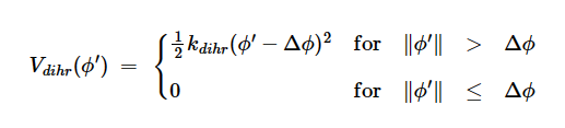
其中,Φ’为参考角Phi,ΔΦ为超出参考角的值dPhi,K_dihr为限制力的大小KFactor。
控制溶剂盒子的几何形状。
体系中分子表面到盒子边界的最小距离(单位 nm)
输出结果包括:
| 输出文件名称 | 说明 |
|---|---|
| system.gro | 体系的分子坐标文件 |
| system_itp.tar.gz | 体系平衡模拟时固定原子位置所施加的力 |
| system.top | 体系的拓扑文件 |
| index.ndx | GROMACS 生成的索引文件,定义体系中原子或残基的分组信息(index groups),用于后续分析或计算时选择特定原子集合 |
GROMACS: High performance molecular simulations through multi-level parallelism from laptops to supercomputers. M. J. Abraham, T. Murtola, R. Schulz, S. Páll, J. C. Smith, B. Hess, E. Lindahl, SoftwareX, 1, (2015), 19-25. DOI: 10.1016/j.softx.2015.06.001
Solvates an MD system by adding a water box and ions.
Input receptor topology file, which can be generated by the GMX Receptor Parameterization module.
Input receptor structure file, which can be generated by the GMX Receptor Parameterization module.
Input receptor parameter (compressed) file, which can be generated by the GMX Receptor Parameterization module.
Input ligand structure (compressed) file, which can be generated by the GMX Ligand Parameterization module.
Input ligand parameter (compressed) file, which can be generated by the GMX Ligand Parameterization module.
Ions to be added. Supports sodium (NA), potassium (K), chloride (CL), calcium (CA), magnesium (MG), and zinc (ZN). To add multiple ion types simultaneously, separate them with a colon :, e.g. NA:K:MG.
Number of ions to be added. When adding multiple ion types, this corresponds to the Ions parameter and should also be colon-separated, e.g. 15:20:30.
Note: Choose either Number of Ions or Concentration of Ions; do not provide both.
Concentration of ions to be added, in mol/L. When adding multiple ion types, this corresponds to the Ions parameter and should also be colon-separated, e.g. 0.15:0.3:0.1.
Note: Choose either Number of Ions or Concentration of Ions; do not provide both.
Output topology file for the entire system.
Output structure file for the entire system.
Output parameter (compressed) file for the entire system.
Distance restraints, effective only when Disre is not set to no. Format:
[AtomIndex1] [AtomIndex2] [Type] [Index] [Type] [Low] [Up1] [Up2] [Factor]
AtomIndex1 and AtomIndex2: Atom indices in system.gro.Type: Restraint type, typically set to 1. See Table 1 for restraint types.Index: Calculation order.Low, Up1, Up2: Distance limits between atoms. Distances between Low and Up1 are unrestricted, but must not exceed Up2. Unit: nm.Factor: Multiplier. The restraint force is calculated as Factor × “Disre Force Constant”. Unit: kJ/mol/nm².Example:
10 16 1 0 1 0.0 0.3 0.4 1.0
10 46 1 1 1 0.0 0.3 0.4 1.0
16 22 1 2 1 0.0 0.3 0.4 2.5
Table 1: Three GROMACS restraint types for atom pairs
| Type Code | Restraint Type | Usage |
|---|---|---|
| 1 | Complex NMR distance restraints | Use when Disre Type is ensemble, i.e., non-bonded interactions set to 1. |
| 6 | Simple harmonic restraints | Use when Disre Type is simple, i.e., intramolecular bonded interactions; can be set to 6 or 10. |
| 10 | Piecewise linear/harmonic restraints | Use when Disre Type is simple, i.e., intramolecular bonded interactions; can be set to 6 or 10. |
Angle restraints define the angle between two atom pairs, effective only when Disre is not set to no. Format:
[AtomIndex1] [AtomIndex2] [AtomIndex3] [AtomIndex4] [Type] [Theta0] [Force Constant] [Multiplicity]
AtomIndex1–AtomIndex2: First atom pair.AtomIndex3–AtomIndex4: Second atom pair.Type: Unused; set to 1.Theta0: Restrained angle. Unit: deg.Force Constant: Restraint force constant. Unit: kJ/mol.Multiplicity: Multiplicity.Example:
2642 2643 2635 2652 1 67.0 1500 1
Dihedral angle restraints, effective only when Disre is not set to no. Format:
[AtomIndex1] [AtomIndex2] [AtomIndex3] [AtomIndex4] [Type] [Label] [Phi] [dPhi] [KFactor] [Power]
AtomIndex1–AtomIndex4: Atom indices forming the dihedral angle.Type: Restraint function type, always 1.Label: Unused.Phi: Reference angle.dPhi: Tolerance beyond the reference angle. Unit: deg.KFactor: Multiplier. The restraint force is calculated as KFactor × “Disre Force Constant”. Unit: kJ/mol/rad².Power: Unused.Example:
2642 2643 2635 2652 1 67.0 1500 1
The restraint potential is shown below:
Where Φ′ is the reference angle Phi, ΔΦ is the deviation dPhi, and K_dihr is the restraint force magnitude KFactor.
Controls the geometry of the solvent box.
Minimum distance from the molecular surface to the box boundary. Unit: nm.
Output files include:
| Output Filename | Description |
|---|---|
system.gro |
Molecular coordinates file of the system. |
system_itp.tar.gz |
Forces applied to fix atom positions during system equilibration. |
system.top |
Topology file of the system. |
index.ndx |
GROMACS-generated index file defining atom or residue groups (index groups) in the system, used for selecting specific atom sets in subsequent analyses or calculations. |
GROMACS: High performance molecular simulations through multi-level parallelism from laptops to supercomputers. M. J. Abraham, T. Murtola, R. Schulz, S. Páll, J. C. Smith, B. Hess, E. Lindahl, SoftwareX, 1, (2015), 19-25. DOI: 10.1016/j.softx.2015.06.001

通过序列比对在人类生殖系数据库中搜索与目标抗体序列最接近的同源模板,输出对应的模板序列以及序列一致性信息。
抗体的序列(纯序列信息,非FASTA格式文件)。
抗体编号类型:kabat、chothia、imgt。
输出同源性最高的n条序列。
抗体的序列文件,FASTA格式。
抗体编号类型:kabat、chothia、imgt。
输出同源性最高的n条序列。
| 输出参数 | 输出文件名称 | 说明 |
|---|---|---|
| Hits Sequence | hits.fasta | 包含同源性最高的n条序列的序列文件 |
| Result | result.json | 包含找到的Germline模板以及序列的一致性信息 |
抗体常用的germline模板:
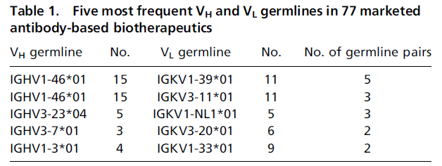
临床后期及已上市抗体的germline配对分布情况(统计自Adimab数据集):
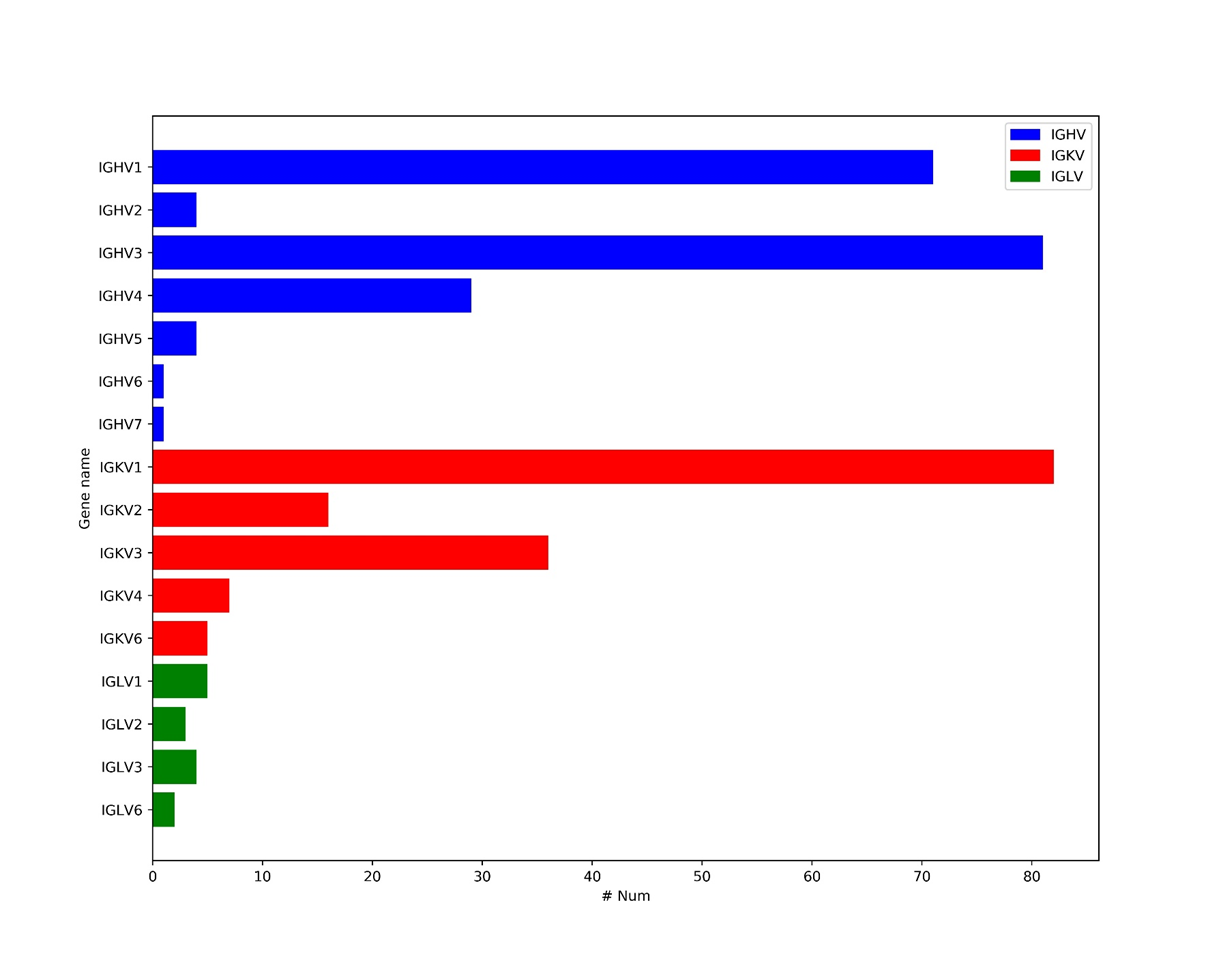
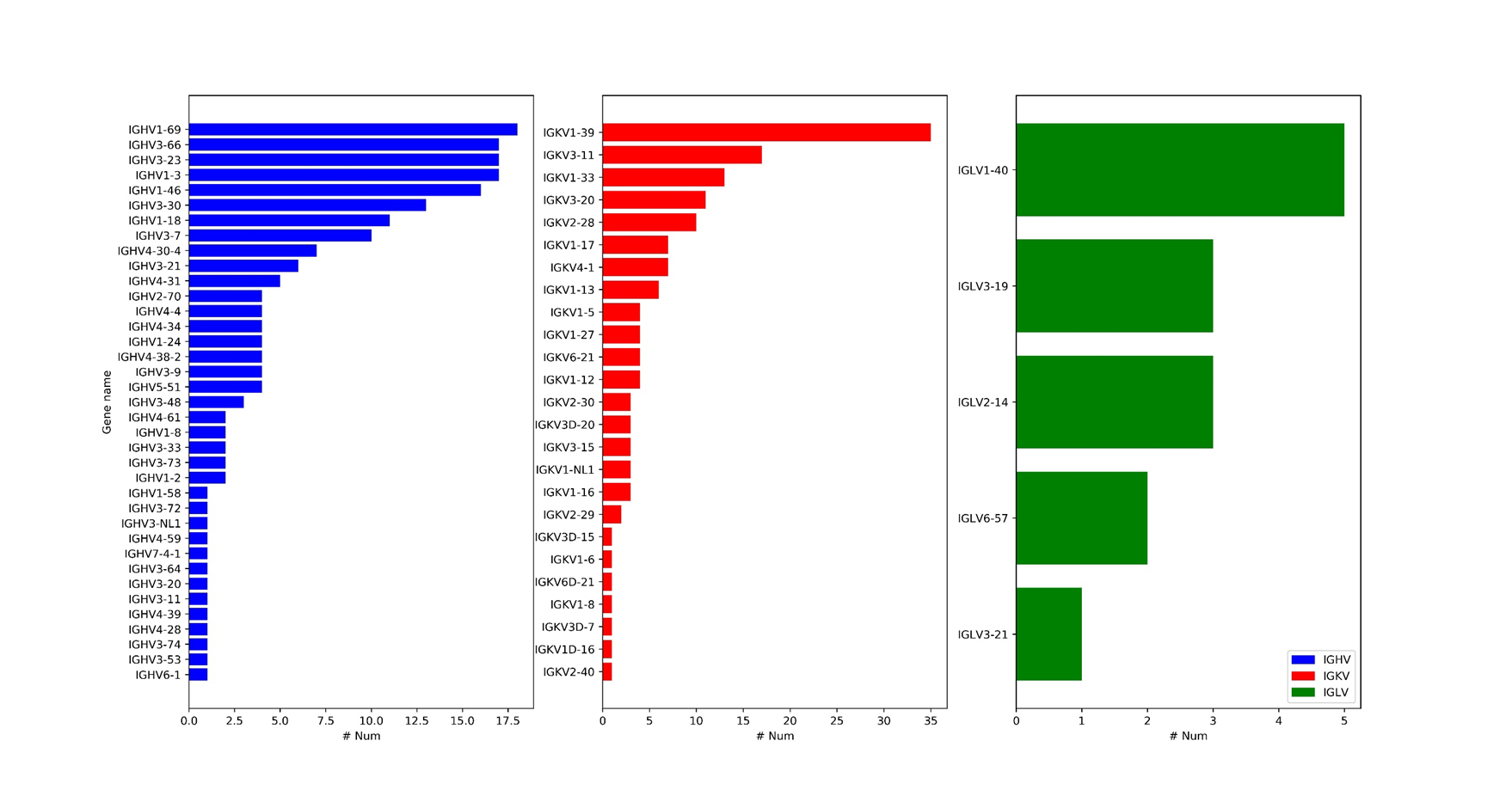
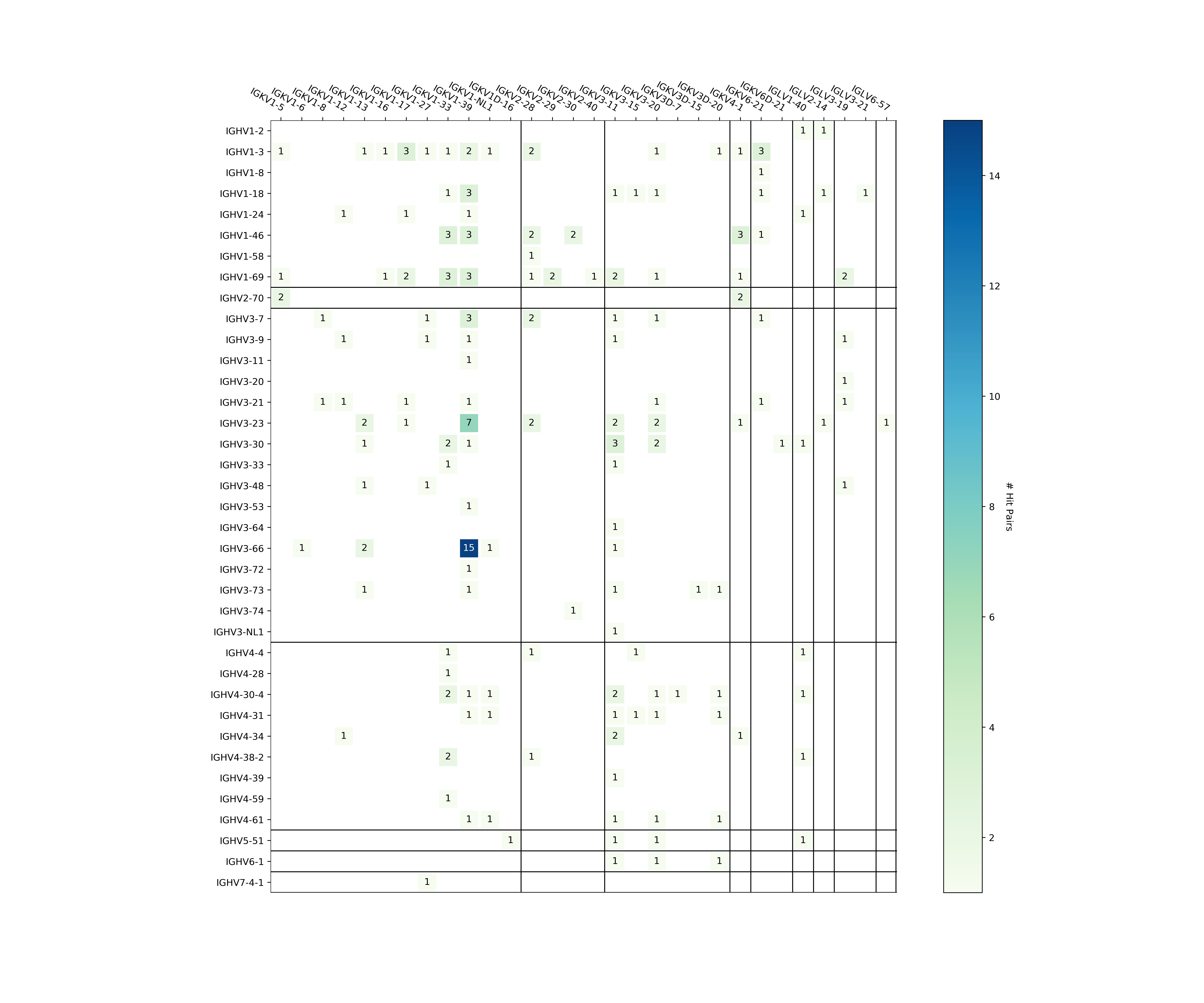
This module performs sequence alignment to search for the closest homologous template in the human germline database for a given target antibody sequence. It outputs the corresponding template sequence along with sequence similarity information.
The antibody sequence (pure sequence information, not in FASTA format).
Type of antibody numbering: kabat, chothia, imgt.
Number of top hits to output.
Antibody sequence file in FASTA format.
Type of antibody numbering: kabat, chothia, imgt.
Number of top hits to output.
| Output Parameter | Output File Name | Description |
|---|---|---|
| Hits Sequence | hits.fasta | File containing the top n sequences with the highest homology |
| Result | result.json | File containing the found Germline template and sequence similarity information |
Commonly used germline templates for antibodies:
Distribution of germline pairing for late-stage and marketed antibodies (statistics from the Adimab dataset):
Grafting模块是移植抗体的CDR到特定的框架区模板上,通常用于人源化设计。版本:v2.4
抗体序列文件,FASTA格式
抗体编号规则:kabat,imgt,chothia
指定输出抗体graft后的序列文件名称,FASTA格式
指定输出graft策略文件,JSON格式
指定输出抗体FR区序列比对同源性打分文件
指定轻链或重链使用特定germline模板,也可都指定,写法如下:
seq_name1:germline_name1,seq_name2:germline_name2
其中链名来自于流程第一步输入的fasta文件。
例1:以下语句为链"Infliximab.H"指定了模板"IGHV3-7*01":
Infliximab.H:IGHV3-7*01
例2:以下语句为两条链分别指定了模板:
Infliximab.H:IGHV3-7*01,Infliximab.L:IGKV1-39*01
指定抗体可变区 V 基因 的参考模板序列,FASTA格式。
指定抗体可变区 J 基因 的参考模板序列,FASTA格式。
指定输出FR区序列比对结果文件,FASTA格式
指定输出命中序列的数目
输出结果包括:
| 输出文件名称 | 说明 |
|---|---|
| germline_hits.fasta | 输出FR区序列比对结果文件 |
| germline_score.json | 输出抗体FR区序列比对同源性打分文件 |
| grafted.fasta | 输出抗体graft后的序列文件名称 |
| graft_policy.json | 输出graft策略文件 |
The Grafting module is used to graft the CDRs of an antibody onto a specific framework region template, typically used for humanization design. Version: v2.4
Antibody sequence file in FASTA format.
Antibody numbering rule: kabat, imgt, chothia.
Specify the output file name for the grafted antibody sequence in FASTA format.
Specify the output grafting strategy file in JSON format.
Specify the output file for the homology scores of the antibody FR region sequences.
Specify the specific germline template to be used for the light chain or heavy chain, or both, in the format:
seq_name1:germline_name1,seq_name2:germline_name2
Where the chain names come from the FASTA file input in the first step of the process.
Example 1: The following statement specifies the template “IGHV3-7*01” for the chain “Infliximab.H”:
Infliximab.H:IGHV3-7*01
Example 2: The following statement specifies templates for two chains separately:
Infliximab.H:IGHV3-7*01,Infliximab.L:IGKV1-39*01
Specify the reference template sequence of the antibody V gene in FASTA format.
Specify the reference template sequence of the antibody J gene in FASTA format.
Specify the output file for the FR region sequence alignment results in FASTA format.
Specify the number of sequences to output.
The output includes:
| Output File Name | Description |
|---|---|
| germline_hits.fasta | Output file for FR region sequence alignment results |
| germline_score.json | Output file for homology scores of the antibody FR region sequences |
| grafted.fasta | Output file name for the grafted antibody sequence |
| graft_policy.json | Output file for the grafting strategy |
该模块基于Pythia模型实现,该模型是一种针对零样本 ∆∆G 预测量身定制的自监督图神经网络。
蛋白质突变效应预测是解码分子进化机制、优化蛋白质工程改造的关键物理量。然而,传统预测方法面临两大挑战:一是基于物理力场的计算方法(如自由能微扰)计算复杂度高,难以满足大规模筛选需求;二是依赖于实验数据的监督学习方法易受训练集偏差影响,泛化能力受限。
为了应对这些问题,研究团队提出了Pythia框架,它结合了图神经网络与注意力机制,能够直接从蛋白质的三维结构中学习氨基酸之间的相互作用。通过这种“零监督”预训练策略,Pythia突破了传统方法对标记数据的依赖,成功捕捉了蛋白质折叠过程中隐藏的物理化学约束规律。
Pythia的模型架构采用了将蛋白质局部结构转化为k近邻图的方式,每个氨基酸作为节点,通过欧几里得距离连接其32个最近的氨基酸。节点的特征包括氨基酸类型以及主链的二面角,边的特征则涉及主链原子之间的距离、序列位置和链信息。通过消息传递神经网络(MPNN)架构,Pythia可以高效地更新每个氨基酸节点的信息,并对突变的稳定性变化进行准确预测。
与传统的基于物理力场的方法相比,Pythia能够在单核计算中实现每分钟预测约50,000个突变,速度提升了5个数量级。其在标准测试集S2648上的Spearman相关系数为0.616,Pearson相关系数为0.598,表现优于现有的所有对比模型。这一进展为大规模蛋白质序列空间扫描提供了强大的计算支持,能够处理多达2600万个高质量蛋白质结构数据,显著加深了我们对蛋白质序列空间的理解。
在实验验证中,Pythia表现出了比传统能量函数方法高出一倍的成功率,充分证明了其在实际应用中的可靠性。同时,Pythia的可解释性也为蛋白质工程提供了宝贵的生物学见解,使其更易于应用于复杂的蛋白质工程任务。
模型架构:Pythia将蛋白质局部结构转换为k近邻图,其中每个氨基酸作为一个节点,并通过欧几里得距离连接其32个最近的氨基酸。节点的特征包括氨基酸类型和主链的二面角(φ、ψ、ω),边的特征包括主链原子之间的距离、序列位置和链信息。
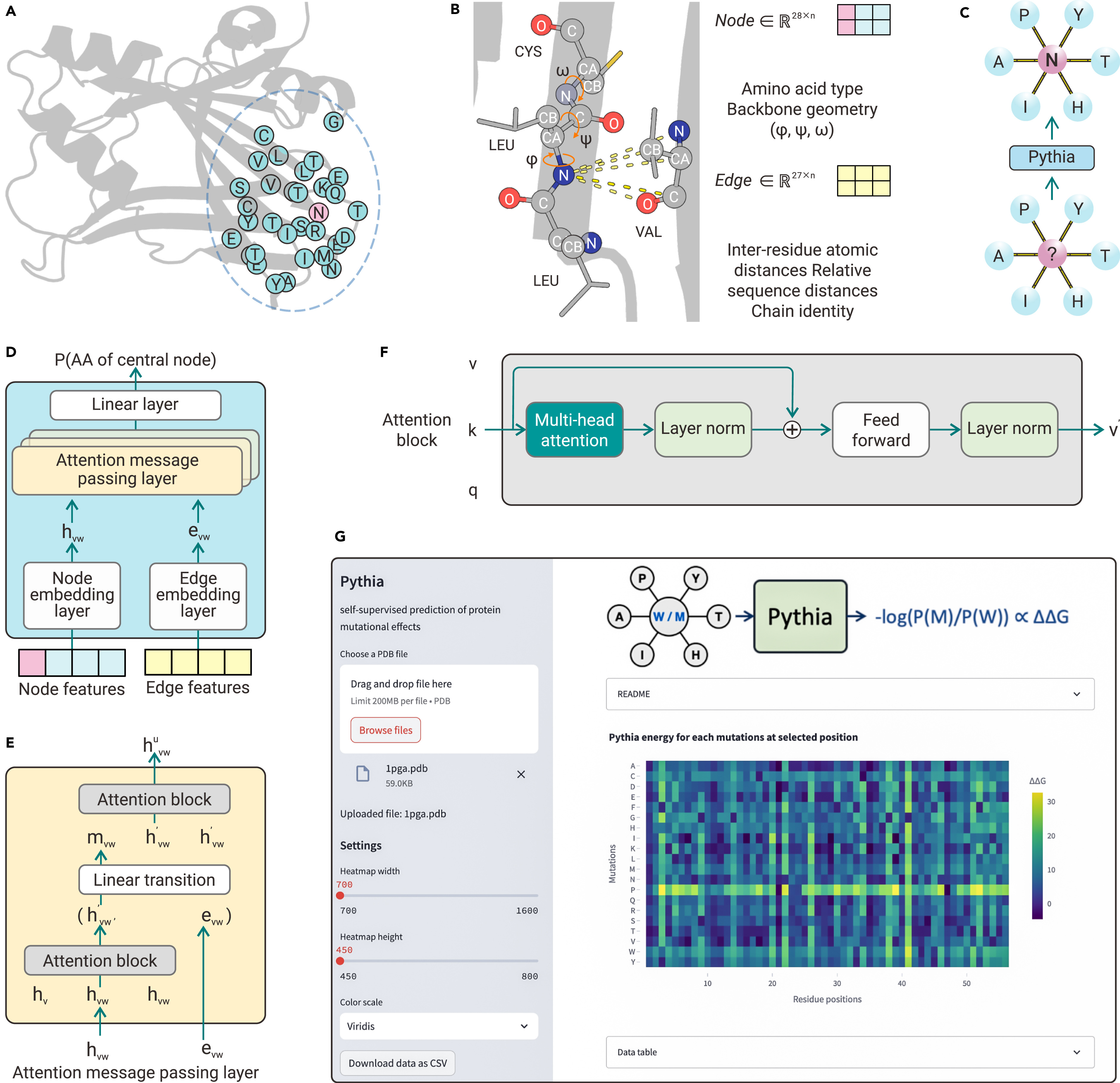
训练目标:Pythia的训练目标是预测中心节点的自然氨基酸类型,使用来自节点和边的信息。
消息传递神经网络(MPNN):Pythia采用消息传递神经网络(MPNN)架构,具体为带有注意力机制的消息传递层(AMPL)。在每个AMPL层中,顶点表示通过注意力块更新,然后与边表示连接以派生消息表示,最终通过另一个注意力块进一步细化节点表示。
损失函数:通过估计特定位置处每个氨基酸的概率来实现ΔΔG的预测。
在与其他自监督预训练模型和基于力场的方法的比较基准中,Pythia以极高的相关性超越其他同类算法,同时以最少的参数运行,使得计算速度显着加快,高达105倍。Pythia的功效通过其在预测柠檬烯环氧水解酶 (LEH) 的热稳定突变中的应用得到证实,实验成功率显着提高。
S2648数据集上的性能:Pythia在S2648数据集上的Spearman相关系数为0.616,Pearson相关系数为0.598,优于所有测试的模型。
S669数据集上的性能:在S669数据集上,Pythia的Spearman相关系数为0.66,在所有评估的方法中表现最佳。
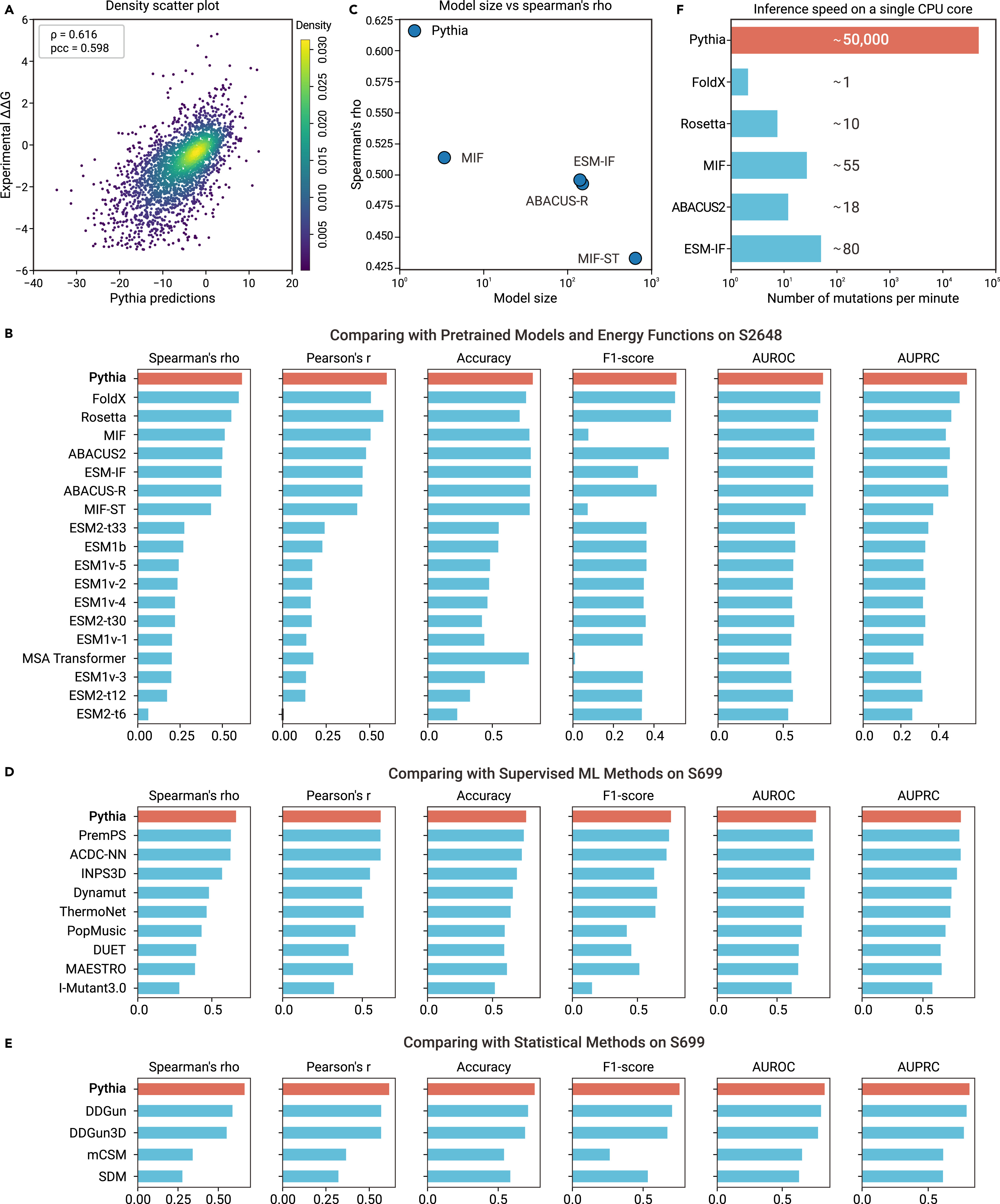
大规模数据集上的性能:在一个包含约100万个突变的百万级数据集上,Pythia的Spearman相关系数为0.602,Pearson相关系数为0.633,AUROC为0.83,AUPRC为0.88。
计算速度:Pythia的计算速度比传统的力场方法快105倍,能够在20秒内完成S2648数据集的计算,单核速度约为50,000个突变/分钟。
蛋白结构文件,PDB格式。不支持含有非标准氨基酸的蛋白。
指定要突变扫描的链名,可多链,用英文逗号分隔,如:A,B,默认为空,表示全部链都扫描。
抗体编号规则,支持Kabat, Chothia和IMGT,默认为Kabat。
指定输出能量最优的前N个突变对应的序列,默认为100。
输出文件名称,默认mutation_energy.csv。
特定格式化的输出文件名称,默认mutation_energy_fmt.csv。
输出TopN对应的突变链的序列,默认为mutant_seqs.fasta。
输出TopN对应的复合物序列,复合物中各链之间用分号:分隔(Boltz2结构预测的批量模式),默认为mutant_seqs_complex.fasta。
备注:当前24GB的GPU显存支持计算的残基数量在2000个左右。
输出mutation_energy.csv结果文件,包含以下信息:
| 字段名称 | 说明 |
|---|---|
| Chain | 链名称,如:'A’表示A链 |
| Mutation | 单点突变信息,如:'G1A’表示该链中,残基位置编号为1的残基甘氨酸G,突变为丙氨酸A,残基位置编号从1开始按顺序编号(非PDB文件中的残基序号) |
| Energy | 突变对应的能量变化,负值表示突变使得体系能量降低,体系变得更稳定。负得越多表示稳定性提升越多 |
输出mutation_energy_fmt.csv结果文件,包含如下信息:
| 字段名称 | 说明 |
|---|---|
| Chain | PDB结构中的链名称 |
| WT | PDB结构中的初始AA |
| Pos | AA位置编号,从1开始 |
| Consensus | 该位置出现能量最优的AA |
| L,A,G,V… | 该位置每种AA对应的能量变化值,变化值为负时,表示更稳定,负得越多,越稳定 |
输出结果对应的热图mutation_energy_[chain].png
输出TopN对应的突变链的序列mutant_seqs.fasta。
输出TopN对应的复合物序列,复合物中各链之间用冒号:分隔(Boltz2结构预测的批量模式)mutant_seqs_complex.fasta。
This module is implemented based on the Pythia model, which is a self-supervised graph neural network specifically designed for zero-shot ∆∆G prediction.
Predicting the effects of protein mutations is a key factor in decoding molecular evolution mechanisms and optimizing protein engineering modifications. However, traditional prediction methods face two major challenges: first, computational methods based on physical force fields (such as free energy perturbation) have high computational complexity, making them unsuitable for large-scale screening; second, supervised learning methods that rely on experimental data are susceptible to training set biases, limiting their generalization ability.
To address these issues, the research team proposed the Pythia framework, which combines graph neural networks with attention mechanisms to learn interactions between amino acids directly from the three-dimensional structure of proteins. Through this “zero-supervision” pre-training strategy, Pythia overcomes the traditional methods’ dependence on labeled data and successfully captures the hidden physicochemical constraints in the protein folding process.
The architecture of Pythia converts the local structure of proteins into k-nearest neighbor graphs, where each amino acid acts as a node connected to its 32 nearest amino acids based on Euclidean distance. Node features include amino acid type and backbone dihedral angles, while edge features involve distances between backbone atoms, sequence positions, and chain information. Using a message-passing neural network (MPNN) architecture, Pythia efficiently updates information for each amino acid node and accurately predicts changes in mutation stability.
Compared to traditional physical force field-based methods, Pythia can predict approximately 50,000 mutations per minute on a single-core processor, achieving a speed increase of five orders of magnitude. On the standard test set S2648, it achieves a Spearman correlation coefficient of 0.616 and a Pearson correlation coefficient of 0.598, outperforming all existing comparative models. This advancement provides powerful computational support for large-scale scanning of protein sequence space, capable of handling up to 26 million high-quality protein structure data points, significantly deepening our understanding of protein sequence space.
In experimental validation, Pythia demonstrated a success rate twice as high as traditional energy function methods, fully proving its reliability in practical applications. Additionally, Pythia’s interpretability offers valuable biological insights for protein engineering, making it more applicable to complex protein engineering tasks.
Model Architecture: Pythia transforms the local structure of proteins into a k-nearest neighbor graph, where each amino acid is represented as a node, connected to its 32 nearest amino acids by Euclidean distance. The features of the nodes include the amino acid type and the backbone dihedrals (φ, ψ, ω), while the features of the edges include the distances between backbone atoms, sequence positions, and chain information.
Training Objective: The training objective of Pythia is to predict the natural amino acid type of the central node, using information from both nodes and edges.
Message Passing Neural Network (MPNN): Pythia employs a message passing neural network (MPNN) architecture, specifically an Attention-based Message Passing Layer (AMPL). In each AMPL layer, the vertices are updated through an attention block, and then connected to edge representations to derive message representations, which are further refined through another attention block.
Loss Function: The prediction of ΔΔG is achieved by estimating the probability of each amino acid at specific positions.
In benchmark comparisons with other self-supervised pre-training models and force-field-based methods, Pythia outperforms other similar algorithms with high correlation while operating with minimal parameters, significantly accelerating computational speed by up to 105 times. The effectiveness of Pythia is demonstrated through its application in predicting thermally stable mutations of limonene epoxide hydrolase (LEH), with a notable increase in experimental success rates.
Performance on the S2648 Dataset: Pythia achieves a Spearman correlation coefficient of 0.616 and a Pearson correlation coefficient of 0.598 on the S2648 dataset, outperforming all tested models.
Performance on the S669 Dataset: On the S669 dataset, Pythia achieves a Spearman correlation coefficient of 0.66, performing the best among all evaluated methods.

Performance on Large-scale Datasets: On a large dataset containing approximately 1 million mutations, Pythia achieves a Spearman correlation coefficient of 0.602, a Pearson correlation coefficient of 0.633, an AUROC of 0.83, and an AUPRC of 0.88.
Computational Speed: Pythia is 105 times faster than traditional force-field methods, capable of completing calculations on the S2648 dataset in 20 seconds, with a single-core speed of approximately 50,000 mutations per minute.
Protein structure file in PDB format. Proteins containing non-standard amino acids are not supported.
Specify the chain names to be scanned for mutations. Multiple chains can be listed, separated by commas, e.g., A,B. The default is empty, which means all chains will be scanned.
Antibody numbering schemes, supporting Kabat, Chothia, and IMGT. The default scheme is Kabat.
Specify the sequences corresponding to the top N mutations with the optimal energy. The default value is 100.
Output file name, mutation_energy.csv is the default.
Formatted output file name, mutation_energy_fmt.csv is the default.
Output the sequences of the mutation chains corresponding to TopN.
Output the sequences of the complexes corresponding to TopN. The chains within the complexes are separated by semicolons (;) (for batch mode structure prediction by Boltz2).
Outputs a mutation_energy.csv file containing the following information:
| Field Name | Description |
|---|---|
| Chain | Chain name, e.g., ‘A’ represents chain A |
| Mutation | Single point mutation information, e.g., ‘G1A’ indicates that in this chain, the residue at position 1, Glycine (G), is mutated to Alanine (A), with residue positions numbered sequentially starting from 1 (not the residue numbering in the PDB file) |
| Energy | The energy change associated with the mutation; negative values indicate that the mutation lowers the system’s energy, making it more stable. The more negative the value, the greater the increase in stability. |
The heatmap output mutation_energy_[chain].png
Output the sequences of the mutation chains corresponding to TopN. mutant_seqs.fasta
Output the sequences of the complexes corresponding to TopN. The chains within the complexes are separated by : (for batch mode structure prediction by Boltz2). mutant_seqs_complex.fasta
Mutation Energy of Binding (Pythia-PPI)模块基于Pythia-PPI模型实现,该模型基于深度学习,结合了多任务学习和自蒸馏策略,以克服实验数据稀缺的瓶颈,并提高预测准确性。Pythia-PPI由两个模块组成:预训练的结构图编码器模块和ΔΔG预测模块。该模型使用k-最近邻(k-NN)图将蛋白质或蛋白质-蛋白质复合物的局部结构转换为图表示,每个氨基酸作为一个节点,与其32个最近的氨基酸基于C-alpha原子的欧几里得距离建立连接。输入的结构图编码器结合了氨基酸类型的一热编码,以及使用正弦和余弦函数表示的主链二面角(φ、ψ和ω)作为节点特征。边特征则考虑了五个主链原子(C-alpha、C、N、O和C-beta)之间的距离,以及序列位置和链信息。通过结构图编码器,节点和边输入特征被转换为嵌入,这些嵌入与预训练模块中的氨基酸概率相结合,形成ΔΔG预测模块的输入向量。Pythia-PPI采用迁移学习和多任务学习相结合的方法,共享结构编码器层以预测突变对PPI结合亲和力和蛋白质稳定性的影响。
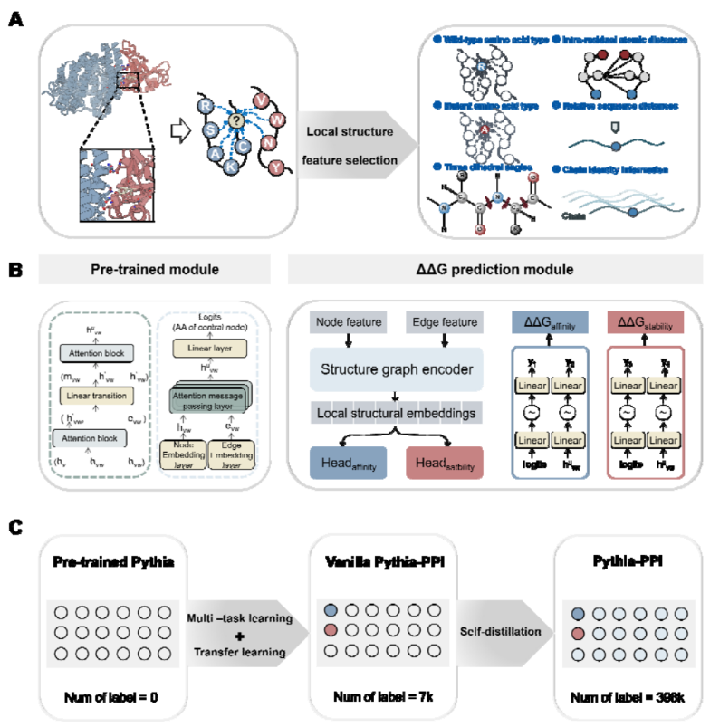
使用了SKEMPI数据集进行基准测试,并与其他方法进行了比较。结果显示,Pythia-PPI在SKEMPI数据集上的皮尔逊相关系数从0.6447提高到0.7850,在病毒-受体数据集上的皮尔逊相关系数从0.3654提高到0.6051。这些结果表明Pythia-PPI是一个分析蛋白质-蛋白质相互作用适应性景观的有力工具。
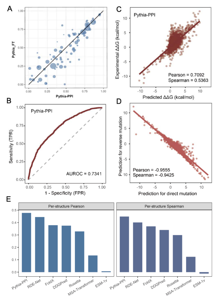
蛋白复合物结构文件,PDB格式。不支持含有非标准氨基酸的蛋白。
指定要突变扫描的链名,可多链,用英文逗号分隔,如:A,B,默认为空,表示全部链都扫描。
抗体编号规则,支持Kabat, Chothia和IMGT,默认为Kabat。
指定输出能量最优的前N个突变对应的序列,默认为100。
输出文件名称,默认mutation_ddg.csv。
特定格式化输出的结果文件名称,默认mutation_ddg_fmt.csv。
输出TopN对应的突变链的序列,默认为mutant_seqs.fasta。
输出TopN对应的复合物序列,复合物中各链之间用分号:分隔(Boltz2结构预测的批量模式),默认为mutant_seqs_complex.fasta。
备注:当前24GB的GPU显存支持计算的残基数量在1500个左右。
输出mutation_ddg.csv结果文件,包含以下信息:
| 字段名称 | 说明 |
|---|---|
| Chain | 链名称,如:'A’表示A链 |
| Mutation | 单点突变信息,如:'G1A’表示该链中,残基位置编号为1的残基甘氨酸G,突变为丙氨酸A,残基位置编号从1开始按顺序编号(非PDB文件中的残基序号) |
| Energe(Pythia-PPI) | 突变对应的结合自由能ddG变化,负值表示突变使得亲和力变高,负得越多表示亲和力提升越多 |
输出mutation_ddg_fmt.csv结果文件,包含如下信息:
| 字段名称 | 说明 |
|---|---|
| Chain | PDB结构中的链名称 |
| WT | PDB结构中的初始AA |
| Pos | AA位置编号,从1开始 |
| Consensus | 该位置出现能量最优的AA |
| L,A,G,V… | 该位置每种AA对应的能量变化值,变化值为负时,表示更稳定,负得越多,越稳定 |
输出结果对应的热图mutation_ddg_[chain].png
输出TopN对应的突变链的序列mutant_seqs.fasta。
输出TopN对应的复合物序列mutant_seqs_complex.fasta,复合物中各链之间用冒号:分隔(Boltz2结构预测的批量模式)。
The Mutation Energy of Binding (Pythia-PPI) module is implemented based on the Pythia-PPI model, which utilizes deep learning and combines multi-task learning with a self-distillation strategy to overcome the bottleneck of scarce experimental data and improve prediction accuracy. Pythia-PPI consists of two modules: a pre-trained structural graph encoder module and a ΔΔG prediction module. The model uses a k-nearest neighbors (k-NN) graph to convert the local structure of proteins or protein-protein complexes into a graph representation, where each amino acid is represented as a node, connected to its 32 nearest amino acids based on the Euclidean distance of C-alpha atoms. The input structural graph encoder combines one-hot encoding of amino acid types with backbone dihedrals (φ, ψ, and ω) represented using sine and cosine functions as node features. Edge features take into account the distances between five backbone atoms (C-alpha, C, N, O, and C-beta), as well as sequence positions and chain information. Through the structural graph encoder, the input features for nodes and edges are transformed into embeddings, which are combined with amino acid probabilities from the pre-trained module to form the input vector for the ΔΔG prediction module. Pythia-PPI employs a combination of transfer learning and multi-task learning, sharing structural encoder layers to predict the effects of mutations on PPI binding affinity and protein stability.
Benchmarking was conducted using the SKEMPI dataset and compared with other methods. The results show that Pythia-PPI improved the Pearson correlation coefficient from 0.6447 to 0.7850 on the SKEMPI dataset, and from 0.3654 to 0.6051 on the virus-receptor dataset. These results indicate that Pythia-PPI is a powerful tool for analyzing the adaptive landscape of protein-protein interactions.

Protein complex structure file in PDB format. Proteins containing non-standard amino acids are not supported.
Specify the chain names to be scanned for mutations. Multiple chains can be listed, separated by commas, e.g., A,B. The default is empty, which means all chains will be scanned.
Antibody numbering schemes, supporting Kabat, Chothia, and IMGT. The default scheme is Kabat.
Specify the sequences corresponding to the top N mutations with the optimal energy. The default value is 100.
Output file name, mutation_ddg.csv is the default.
Formatted output file name, mutation_ddg_fmt.csv is the default.
Output the sequences of the mutation chains corresponding to TopN.
Output the sequences of the complexes corresponding to TopN. The chains within the complexes are separated by semicolons (;) (for batch mode structure prediction by Boltz2).
Outputs a mutation_ddg.csv file containing the following information:
| Field Name | Description |
|---|---|
| Chain | Chain name, e.g., ‘A’ represents chain A |
| Mutation | Single point mutation information, e.g., ‘G1A’ indicates that in this chain, the residue at position 1, Glycine (G), is mutated to Alanine (A), with residue positions numbered sequentially starting from 1 (not the residue numbering in the PDB file) |
| Energe(Pythia-PPI) | The change in binding free energy (ddG) corresponding to the mutation; negative values indicate that the mutation increases affinity, with more negative values indicating a greater increase in affinity. |
Outputs a mutation_ddg_fmt.csv file containing the following information:
| Field Name | Description |
|---|---|
| Chain | Chain name in the PDB structure |
| WT | Initial AA in the PDB structure |
| Pos | Position index of the AA, start from 1 |
| Consensus | The AA with the most affinity value at that position |
| L, A, G, V… | The ddg of each AA at that position. Negative values indicate that the mutation increases affinity, with more negative values indicating a greater increase in affinity. |
The heatmap output mutation_ddg_[chain].png
Output the sequences of the mutation chains corresponding to TopN mutant_seqs.fasta.
Output the sequences of the complexes corresponding to TopN mutant_seqs_complex.fasta. The chains within the complex are separated by colons(:) (for batch mode of Boltz2 structure prediction) .

Antibody (Off-) Target Prediction模块对输入的抗体进行潜在靶点预测,基于丰富的抗体-抗原相互作用数据库,寻找与输入抗体在序列及结构上高度相似的一系列抗体。基于相似性原理(相似抗体可能具有相似靶点),这些高度相似的抗体对应的抗原靶点可能是输入抗体的潜在靶点。当前抗体-抗原相互作用数据库包含16万对抗原-抗体复合物,主要来源于文献、专利等开源数据。
待预测靶点的抗体结构文件,PDB格式或CIF格式。
搜索模式,支持4种模式(默认为模式2):
注意: 纳米抗体VHH只能使用模式3或模式4,使用其他模式会提示错误。
保留打分排名最高的前N个结果,默认为50。
物种信息过滤:
输出结果的文件名,默认为pred_hits.csv
结果文件有多个,根据抗体结构来源不同会有不同的预测结果,以及合并后的最终结果。
当前抗体结构来源有2种:实验结构(来自PDB数据库)、Boltz模型预测结构。
结果文件有:
pred_hits_Experimental.csvpred_hits_Boltz.csvpred_hits.csvpred_hits_Experimental.csv,pred_hits_Boltz.csv包含如下信息:
| 字段名 | 说明 |
|---|---|
| Query | 查询抗体结构名称 |
| Database | 抗体结构来源 |
| Antigen Name | 预测的靶点名称 |
| Description | 对数据库结构的描述 |
| Antigen Organism | 靶点的来源物种 |
| Comprehensive Score | 潜在靶点的综合打分,数值在0-1.0之间,越接近1.0,表示成为抗体靶点的可能性越大,默认基于该打分对潜在靶点进行排序。该打分综合了多种结构比对与复合物评价指标。 |
| Alignment TMScore \ Query TMScore \ Target TMScore | TM-score (Template Modeling Score) 是一种结构比对指标,用于衡量两个蛋白质三维结构的相似性,与 RMSD相比,TM-score 更加稳定,对结构长度不敏感,能更准确地反映蛋白质结构的全局相似性。其取值范围在0到1之间,TM-score > 0.5 表示显著相似。其中,Query TMScore指使用查询抗体结构进行长度归一化;Target TMScore指使用数据库抗体结构进行长度归一化;Alignment TMScore指使用查询抗体和数据库抗体的序列匹配区的结构进行长度归一化。 |
| DockQ | 衡量抗体与潜在靶点之间的虚拟结合参数,其值在0-1.0之间,越大表示抗体越能与潜在靶点结合。 |
pred_hits.csv包含信息如下:
| 字段名 | 说明 |
|---|---|
| Query | 查询抗体结构名称 |
| Antigen Name | 预测的靶点名称 |
| Description | 对数据库结构的描述 |
| Antigen Organism | 靶点的来源物种 |
| Comprehensive Score (Boltz) | 基于Boltz预测结构的抗体结构数据库对应的综合打分。 |
| Comprehensive Score (Experimental) | 基于实验结构的抗体结构数据库对应的综合打分。 |
| Comprehensive Score | 不同数据库来源的综合打分平均值,默认基于该打分对潜在靶点进行排序。 |
The Antibody (Off-) Target Prediction module predicts potential targets for the input antibody. Based on a rich database of antibody-antigen interactions, it identifies a series of antibodies that are highly similar to the input antibody in both sequence and structure. Following the principle of similarity (similar antibodies may have similar targets), the antigen targets corresponding to these highly similar antibodies could be potential targets for the input antibody. The current antibody-antigen interaction database contains 160,000 antigen-antibody complexes, primarily sourced from open-source data such as literature and patents.
Antibody structure file for the target to be predicted, in PDB or CIF format.
Search Modes, supporting 4 modes (default is Mode 2):
Retain the top N results with the highest scores, with the default being 50.
Species Information Filtering:
The name of output file, default is “pred_hits.csv”.
There are multiple output files, each corresponding to a different antibody-structure source, plus a final merged result.
Current antibody-structure sources are:
Output files:
Contents of pred_hits_Experimental.csv and pred_hits_Boltz.csv:
| Field | Description |
|---|---|
| Query | Name of the query antibody structure |
| Database | Source of the antibody structure |
| Antigen Name | Predicted target name |
| Description | Description of the database entry |
| Antigen Organism | Species of origin for the predicted target |
| Comprehensive Score | Overall score (0–1.0) for the potential target; closer to 1.0 indicates a higher likelihood of being the antibody’s true target. Targets are ranked by this score by default. The score integrates multiple structural-alignment and complex-quality metrics. |
| Alignment TMScore / Query TMScore / Target TMScore | TM-score (Template Modeling Score) measures global structural similarity between two protein 3-D structures. It is more robust and length-insensitive than RMSD, with values from 0 to 1. TM-score > 0.5 indicates significant similarity. Query TMScore normalizes by query antibody length; Target TMScore normalizes by database antibody length; Alignment TMScore normalizes by the structurally aligned region shared by both antibodies. |
| DockQ | Virtual binding quality score between the antibody and the potential target (0–1.0); higher values suggest stronger predicted binding. |
Contents of pred_hits.csv:
| Field | Description |
|---|---|
| Query | Name of the query antibody structure |
| Antigen Name | Predicted target name |
| Description | Description of the database entry |
| Antigen Organism | Species of origin for the predicted target |
| Comprehensive Score (Boltz) | Comprehensive score derived from the Boltz-predicted structure database |
| Comprehensive Score (Experimental) | Comprehensive score derived from the experimental-structure database |
| Comprehensive Score | Mean of the scores from all sources; targets are ranked by this value by default |
基于TemBERTure开发的Thermostability Prediction是一个用于预测蛋白质热稳定性的深度学习工具,专注于氨基酸序列分析。它包括两个模型:TemBERTureCLS和TemBERTureTm。TemBERTureCLS是一个分类模型,用于预测蛋白质序列的热类别,即判断其是嗜热的还是非嗜热的。TemBERTureTm是一个回归模型,用于根据蛋白质序列预测其熔点温度(Tm)。这两个模型都基于protBERT-BFD语言模型,该模型在大量蛋白质序列数据集上进行了预训练。通过基于适配器的方法进行高效微调,使得TemBERTure能够在不需要广泛重新训练的情况下,稳健地适应特定任务。

TemBERTureCLS与其他常用模型的预测结果比较

TemBERTureTm与其他常用模型的预测结果比较
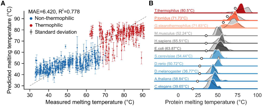
蛋白的序列文件,FASTA格式
默认输出结果文件为predicted_Tm.csv,包含信息如下:
| 字段名称 | 说明 |
|---|---|
| ID | 序列ID |
| Tm | 预测得到的蛋白Melting Temperature ™ 值 |
| Thermostability Type | 预测得到的蛋白热稳定性类别,有两种:Thermophilic与Non-thermophilic |
| Thermophilicity Prediction Score | 预测得到的蛋白嗜热性概率评分,数值在0-1.0之间,越大表示蛋白嗜热的概率越高 |
Thermostability Prediction, developed based on TemBERTure, is a deep learning tool designed to predict protein thermostability, focusing on amino acid sequence analysis. It includes two models: TemBERTureCLS and TemBERTureTm. TemBERTureCLS is a classification model used to predict the thermal category of a protein sequence, determining whether it is thermophilic or non-thermophilic. TemBERTureTm is a regression model used to predict the melting temperature ™ of a protein based on its sequence. Both models are based on the protBERT-BFD language model, which has been pre-trained on a large dataset of protein sequences. By using an adapter-based fine-tuning approach, TemBERTure can efficiently and robustly adapt to specific tasks without the need for extensive retraining.
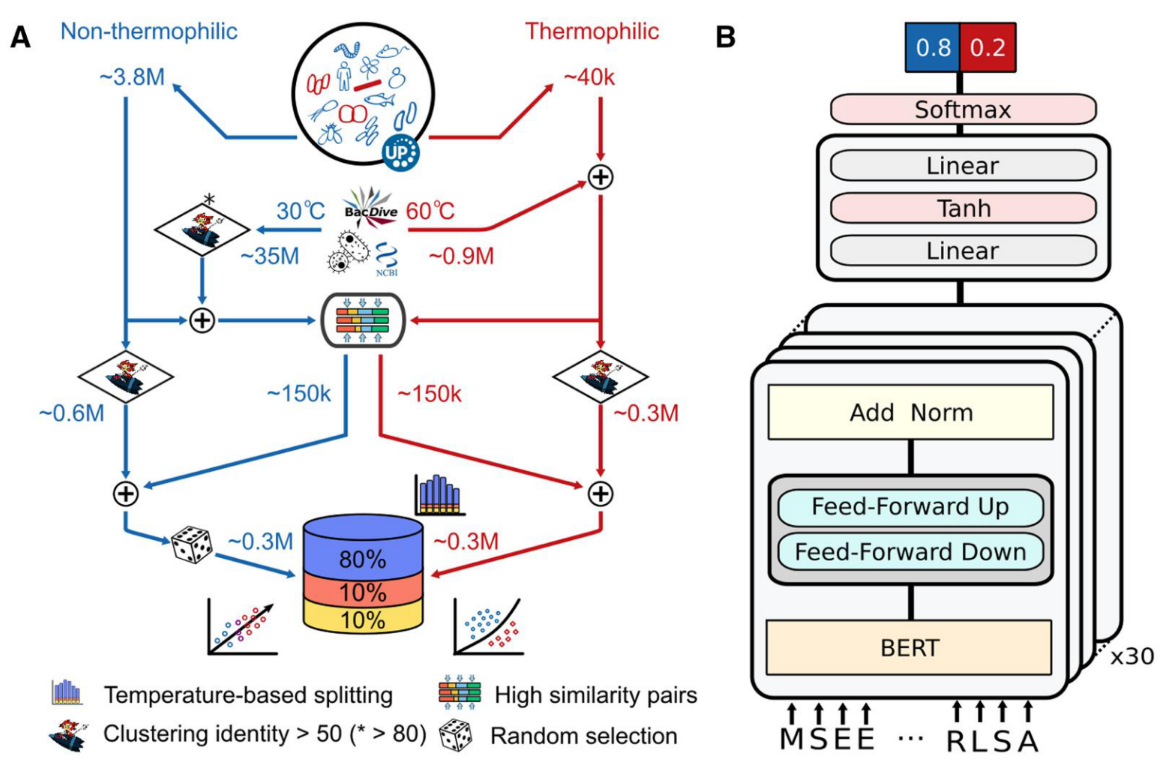
Comparison of TemBERTureCLS with other common models’ prediction results
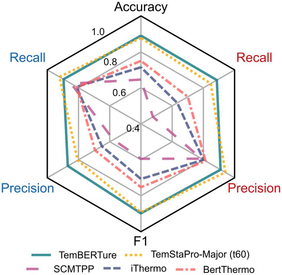
Comparison of TemBERTureTm with other common models’ prediction results

The protein sequence file in FASTA format.
The output result file is predicted_Tm.csv, containing the following information:
| Field Name | Description |
|---|---|
| ID | Sequence ID |
| Tm | Predicted protein Melting Temperature ™ value |
| Thermostability Type | Predicted protein thermostability category: either Thermophilic or Non-thermophilic |
| Thermophilicity Prediction Score | Predicted probability score of protein thermophilicity, ranging from 0 to 1.0, where a higher score indicates a higher likelihood of the protein being thermophilic |

GMX Metadynamics Generation模块是生成可用于Metadynamics模拟的输入文件。
提交模拟体系的gro文件。该文件可以从MD Solvation模块获取。
Metadynamics模拟阶段是否考虑周期性边界条件,yes或者no。
组成集合变量CV的第一个组所包含的原子。
组成集合变量CV的第二个组所包含的原子。
组成集合变量CV的第三个组所包含的原子。
组成集合变量CV的第四个组所包含的原子。
备注:
集合变量DISTANCE对应的成分,其成分有x,y,z和xyz,分别表示计算DISTANCE仅考虑x,y,z维度以及xyz三个维度都考虑,有多个集合变量时用"//"进行分割。
施加的沉积高斯函数的高度,默认1.0
施加的沉积高斯函数的宽度或者标准差,有多个集合变量时用"//"进行分割,默认0.05
施加的沉积高斯函数的频率,默认500,即每500个时间步长进行一次高斯函数沉积
集合变量的边界最小值,有多个集合变量时用"//"进行分割。无默认值时即不考虑边界,此时计算量会增加,强烈建议设置边界。
集合变量的边界最大值,有多个集合变量时用"//"进行分割,无默认值时即不考虑边界,此时计算量会增加,强烈建议设置边界。
集合变量的窗口大小,有多个集合变量时用"//"进行分割,默认等于metad_width的1/5
集合变量的窗口数量,有多个集合变量时用"//"进行分割,默认等于150,CV Space和CV Bin的相乘等于CV Max和CV Min的差值,因此当CV Space和CV Bin同时设置时以对应窗口数最多的为准
是否考虑施加自适应沉积函数, geom或者diff,默认为不填,即不考虑自适应。
施加的自适应高斯函数的宽度或者标准差的最小值,有多个集合变量时用"//"进行分割,默认等于0。
施加的自适应高斯函数的宽度或者标准差的最大值,有多个集合变量时用"//"进行分割,默认等于0。
是否考虑重加权以获得重加权因子,对获得归一化偏势,yes或者no,默认no,即不考虑重加权,一般在体系收敛后才考虑重加权。
计算重加权因子时施加的高斯函数的个数,默认等于50。
计算重加权因子时集合变量的窗口数量,其值不能小于CV Bin的值,有多个集合变量时用"//"进行分割,默认等于CV Bin。
是否考虑回火metadynamics模拟,yes或者no。
回火metadynamics模拟时对应的基础温度,默认等于300K
回火Metadynamics模拟时对应的偏置因子,其值等于(T+deltaT)/T,默认等于1,此时未进行偏置模拟,若进行偏置模拟,偏置因子应大于1
回火Metadynamics模拟时对应的施加的沉积高斯函数的高度,Height=kbDeltaTFrequency*TimeStep/TAU,默认等于0,即直接使用设置的沉积函数的高度代替。
Metadynamics模拟时指定的输出步长,默认100。
Metadynamics模拟时指定的沉积高斯函数的输出文件名。
Metadynamics模拟时指定的集合变量的输出文件名。
Metadynamics模拟时指定的CV Group的输出文件名,该文件中包含所有的CV Group的原子组,用于下一步Metadynamics的输入文件。
Metadynamics模拟时指定的参数的输出文件名,该文件中包含计算时所需的参数,用于下一步Metadynamics的输入文件。
输出结果包括:
| 输出文件名称 | 说明 |
|---|---|
| HILLS.dat | Metadynamics模拟时指定的沉积高斯函数输出 |
| COLVAR.dat | Metadynamics模拟时指定的集合变量的输出 |
| PLUMED.ndx | NDX文件指定的组成集合变量的原子组 |
| PLUMED.dat | 下一步Metadynamics计算所需的参数文件 |
上述两个生成的文件将作为下一步metadynamics模拟的输入文件。
The GMX Metadynamics Generation module is used to generate input files for Metadynamics simulations.
Submit the gro file of the simulation system. This file can be obtained from the MD Solvation module.
Whether to consider periodic boundary conditions during the Metadynamics simulation phase, yes or no.
Atoms included in the first group that makes up the collective variable (CV).
Atoms included in the second group that makes up the collective variable (CV).
Atoms included in the third group that makes up the collective variable (CV).
Atoms included in the fourth group that makes up the collective variable (CV).
Note:
The components corresponding to the DISTANCE collective variable, which can be x, y, z, and xyz, representing calculations of DISTANCE considering only the x, y, z dimensions or all three dimensions, respectively. Use “//” to separate multiple collective variable components.
The height of the deposited Gaussian function, default is 1.0.
The width or standard deviation of the deposited Gaussian function. Use “//” to separate multiple collective variable widths, default is 0.05.
The frequency of depositing the Gaussian function, default is 500, meaning a Gaussian function deposition occurs every 500 time steps.
The minimum boundary value of the collective variable. Use “//” to separate multiple collective variable minimums. If there is no default value, the boundary will not be considered, which will increase the computational load. It is strongly recommended to set boundaries.
The maximum boundary value of the collective variable. Use “//” to separate multiple collective variable maximums. If there is no default value, the boundary will not be considered, which will increase the computational load. It is strongly recommended to set boundaries.
The window size of the collective variable. Use “//” to separate multiple collective variable window sizes, default is 1/5 of metad_width.
The number of windows for the collective variable. Use “//” to separate multiple collective variable bin counts, default is 150. The product of CV Space and CV Bin equals the difference between CV Max and CV Min. Therefore, when both CV Space and CV Bin are set, the one with the highest corresponding window count will prevail.
Whether to consider applying an adaptive deposition function, geom or diff, default is not filled, which means adaptive deposition is not considered.
The minimum width or standard deviation of the applied adaptive Gaussian function. Use “//” to separate multiple collective variable minimums, default is 0.
The maximum width or standard deviation of the applied adaptive Gaussian function. Use “//” to separate multiple collective variable maximums, default is 0.
Whether to consider reweighting to obtain the reweighting factor for normalization of the bias potential, yes or no, default is no, which means reweighting is not considered. Reweighting is generally considered only after the system has converged.
The number of Gaussian functions applied when calculating the reweighting factor, default is 50.
The number of windows for the collective variable when calculating the reweighting factor, which cannot be less than the value of CV Bin. Use “//” to separate multiple collective variable bin counts, default is equal to CV Bin.
Whether to consider simulated annealing in the Metadynamics simulation, yes or no.
The base temperature corresponding to the simulated annealing Metadynamics simulation, default is 300K.
The bias factor corresponding to the simulated annealing Metadynamics simulation, which equals (T + deltaT) / T, default is 1, meaning no bias simulation is performed. If a bias simulation is performed, the bias factor should be greater than 1.
The height of the deposited Gaussian function applied during the simulated annealing Metadynamics simulation, Height = kb * DeltaT * Frequency * TimeStep / TAU, default is 0, meaning the set deposition function height is used directly.
The specified output step length during the Metadynamics simulation, default is 100.
The output file name for the deposited Gaussian function during the Metadynamics simulation.
The output file name for the collective variable during the Metadynamics simulation.
The output file name for the CV Group during the Metadynamics simulation, which contains all the atom groups of the CV Group for the next step’s Metadynamics input file.
The output file name for the parameters during the Metadynamics simulation, which contains the parameters required for calculations for the next step’s Metadynamics input file.
The output results include:
| Output File Name | Description |
|---|---|
| HILLS.dat | Output of the deposited Gaussian function specified during the Metadynamics simulation |
| COLVAR.dat | Output of the collective variable specified during the Metadynamics simulation |
| PLUMED.ndx | NDX file specifying the atom groups that make up the collective variable |
| PLUMED.dat | Parameter file required for the next step of Metadynamics calculation |
The two generated files above will serve as input files for the next step of the Metadynamics simulation.
Free Energy Surface Analysis模块是对基于PLUMED元动力学模拟后得到的模拟结果进行自由能计算。
基于PLUMED元动力学模拟后输出的沉积高斯函数文件,默认为HILLS.dat文件。
对沉积高斯函数文件进行自由能计算时是否考虑直方图分布方法,yes或者no,默认no。
当考虑直方图分布方法时高斯函数的宽度值,有多个集合变量(即CV)时用"//"进行分割,比如0.35//0.35。只有当Histogram值为no时Sigma参数才会生效,当有多个CV而只设置了一个宽度值时,则表示该宽度值适用于所有CV。默认0.05。
CV名称,对沉积高斯函数文件进行自由能计算时只考虑该指定的CV。当不指定CV时则考虑沉积高斯函数文件中包含的所有CV,当指定CV时则不能考虑直方图分布方法。
集合变量的边界最小值,有多个集合变量时用"//"进行分割,比如0.1//0.3,强烈建议设置边界。当有多个CV而只设置了一个边界最小值时,则表示该最小值适用于所有CV。
集合变量的边界最大值,有多个集合变量时用"//"进行分割,比如0.1//0.3,强烈建议设置边界。当有多个CV而只设置了一个边界最大值时,则表示该最大值适用于所有CV。
集合变量的窗口大小,有多个集合变量时用"//"进行分割,比如0.1//0.3。仅当设置了CV Min和CV Max值时,Grid Size才会生效。当有多个CV而只设置了一个窗口大小值时,则表示该窗口大小值适用于所有CV。
集合变量的窗口数量,有多个集合变量时用"//"进行分割,比如150//300。仅当设置了CV Min和CV Max值时,Bin才会生效。当有多个CV而只设置了一个窗口数量值时,则表示该窗口数量值适用于所有CV。Grid Size和Bin相乘等于CV Max和CV Min的差值,因此当Grid Size和Bin同时设置时以对应窗口数最多的为准。
温度,对沉积高斯函数文件进行自由能计算时使用的温度值,默认300K
是否对输出的自由能数据进行归零处理,即将自由能数据进行相对移动以保证最小值移动到0的位置,yes或者no,默认no。
沉积高斯函数的数量,在对沉积高斯函数文件进行自由能计算时,每隔该指定的沉积高斯函数的数量进行一次自由能计算。当不设置该数量值时表示对所有的沉积高斯函数在整体上只进行一次自由能计算。
输出结果文件,文件中包含随CV变化的自由能数据,默认为FES.csv文件。当指定了Stride值时,默认文件为FES.dat.tar.gz。
输出结果包括:
| 输出文件名称 | 说明 |
|---|---|
| FES.csv | 随CV变化的自由能数据文件 |
| FES.dat.tar.gz | 随CV变化的自由能数据压缩文件 |
The Free Energy Surface Analysis module is used to to calculate the free energy based on the simulation results outputed from the metadynamics simulations.
The deposited Gaussian function file outputed from the metadymamics simulations. Default “HILLS.dat”.
Whether considers the Historgram method when calculates the free energy based on the deposited Gaussian function file. “yes” or “no”, default “no”.
Width of Gaussian Function used by the Historgram method, if there are multiple CVs, you can separated them by “//”, such as 0.35//0.35. Only effective when Historgram method is used. When there are multiple CVs and only one width value is set, it means that the width value will be applied to all CVs. Default 0.05.
The specified CV considered in the free energy calculation based on the deposited Gaussian function file. When CV is not specified, all CVs contained in the deposited Gaussian function file will be considered, and when CV is specified, histogram distribution methods cannot be considered.
The minimum boundary value of the collective variable. Use “//” to separate multiple collective variable minimums, such as 0.1//0.3. It is strongly recommended to set boundaries. When there are multiple CVs and only one minimum value is set, it means that the minimum value will be applied to all CVs.
The maximum boundary value of the collective variable. Use “//” to separate multiple collective variable maximums, such as 0.1//0.3. It is strongly recommended to set boundaries. When there are multiple CVs and only one maximum value is set, it means that the maximum value will be applied to all CVs.
The window size of the collective variable. Use “//” to separate multiple collective variable window sizes, such as 0.1//0.3. Only effective when CV Min and CV Max values are set. When there are multiple CVs and only one window size value is set, it means that the window size value will be applied to all CVs.
The window number of the collective variable. Use “//” to separate multiple collective variable bin counts, such as 150//300. Only effective when CV Min and CV Max values are set. When there are multiple CVs and only one window number value is set, it means that the window number value will be applied to all CVs.The product of Grid Size and Bin equals the difference between CV Max and CV Min. Therefore, when both CV Space and CV Bin are set, the one with the highest corresponding window count will prevail.
The temperature value used in the free energy calculation based on the deposited Gaussian function file. Default 300K.
Whether mintozeros the obatined free energy data calculated based on the deposited Gaussian function file. “yes” or “no”, default “no”.
Specified number of the deposition Gauss function. When calculates the free energy based on the deposition Gauss function file, the free energy will be calculated every specified number of the deposition Gauss function. When this stride value is not set, it means that only one free energy calculation is performed for all deposition Gaussian functions as a whole.
The specified output file. The output file contains free energy data that varies with CV. Default FES.csv file. When the Stride value is specified, default FES.dat.tar.gz file.
The output results include:
| Output File Name | Description |
|---|---|
| FES.csv | output file that contains free energy data that varies with CV |
| FES.dat.tar.gz | output tar.gz file that contains free energy data that varies with CV |
MD Clustering是对动力学轨迹进行归簇分析。
MD模拟后得到的路径文件,可以在GMX MD Run (GMX2023)模块或者AlphaAutoMD (GMX2023)模块中获取。
聚类时结构的RMSD截断值(nm)
聚类算法:linkage, jarvis-patrick, monte-carlo, diagonalization, gromos, 默认使用gromos算法。
选择需要计算的结构组别:Backbone,Protein,DNA,RNA,Complex。
可以根据PDB中小分子的名称填写组别名称。
注:其中Complex指的是蛋白-小分子复合物体系。
自定义需要计算的残基编号,连续参数可用“-”表示,不连续残基用逗号隔开,例如:1-10,15
自定义需要计算的原子编号,连续参数可用“-”表示,不连续残基用逗号隔开,例如:1-10,15
每一帧的间隔时间(单位ns)
输出结果包括:
| 输出文件名称 | 说明 |
|---|---|
| clusters.pdb | 差异较大的每个簇的代表性结构 |
| clust-size.xvg | 各个簇的帧数 |
| clust-size.xvg | 各个簇和轨迹帧号的对应关系 |
MD Clustering is a clustering analysis of molecular dynamics trajectories.
Path file obtained after MD simulation, can be obtained from the GMX MD Run (GMX2023) module or the AlphaAutoMD (GMX2023) module.
RMSD cutoff value for clustering (in nm).
Clustering algorithm: linkage, jarvis-patrick, monte-carlo, diagonalization, gromos. The default method is gromos.
Select the structural group for calculation: Backbone, Protein, DNA, RNA, or Complex.
You can also specify the group name based on the small molecule names in the PDB file.
Note: “Complex” refers to protein-small molecule complex systems.
Custom residue numbers for calculation. Use “-” for continuous residues and commas to separate non-continuous residues. For example: 1-10, 15.
Custom atom numbers for calculation. Use “-” for continuous atoms and commas to separate non-continuous atoms. For example: 1-10, 15.
Time interval between frames (in ns).
The output results include:
| Output File Name | Description |
|---|---|
| clusters.pdb | Representative structures of each cluster with significant differences |
| clust-size.xvg | Number of frames in each cluster |
| clust-size.xvg | Correspondence between clusters and trajectory frame numbers |
MD Hbond模板对于指定组别之间的氢键分析。
MD模拟后得到的路径文件,可以在GMX MD Run (GMX2023)模块或者AlphaAutoMD (GMX2023)模块中获取。
选择需要计算的氢键组别1:Protein,DNA,RNA。如果两个组相同则分析的是组内氢键。
可以根据PDB中小分子的名称填写组别名称。
选择需要计算的氢键组别2:Protein,DNA,RNA。如果两个组相同则分析的是组内氢键。
可以根据PDB中小分子的名称填写组别名称。
自定义需要计算的组1残基编号,连续参数可用“-”表示,不连续残基用逗号隔开,例如:1-10,15
自定义需要计算的组1原子编号,连续参数可用“-”表示,不连续残基用逗号隔开,例如:1-10,15
自定义需要计算的组2残基编号,连续参数可用“-”表示,不连续残基用逗号隔开,例如:1-10,15
自定义需要计算的组2原子编号,连续参数可用“-”表示,不连续残基用逗号隔开,例如:1-10,15
每一帧的间隔时间(单位ns)
输出结果包括:
| 输出文件名称 | 说明 |
|---|---|
| hbnum.csv | 氢键分析CSV文件 |
| hbnum.xvg | 氢键分析XVG文件 |
| hbnum.png | 氢键分析PNG文件 |
其中hbnum.csv包括信息如下:
| 字段名称 | 说明 |
|---|---|
| Time (ns) | 时间 |
| Hydrogen bonds | 氢键数目 |
| Pairs within 0.35 nm | 两个组相距0.35nm内的接触的原子数目 |
MD Hbond template is used for analyzing hydrogen bonds between specified groups.
Path file obtained after MD simulation, can be obtained from the GMX MD Run (GMX2023) module or the AlphaAutoMD (GMX2023) module.
Select the hydrogen bond group 1 for calculation: Protein, DNA, RNA. If both groups are the same, it analyzes intra-group hydrogen bonds. You can specify group names based on the names of small molecules in the PDB file.
Select the hydrogen bond group 2 for calculation: Protein, DNA, RNA. If both groups are the same, it analyzes intra-group hydrogen bonds. You can specify group names based on the names of small molecules in the PDB file.
Custom residue numbers for group 1 calculation. Use “-” for continuous residues and commas to separate non-continuous residues. For example: 1-10, 15.
Custom atom numbers for group 1 calculation. Use “-” for continuous atoms and commas to separate non-continuous atoms. For example: 1-10, 15.
Custom residue numbers for group 2 calculation. Use “-” for continuous residues and commas to separate non-continuous residues. For example: 1-10, 15.
Custom atom numbers for group 2 calculation. Use “-” for continuous atoms and commas to separate non-continuous atoms. For example: 1-10, 15.
Time interval between frames (in ns).
The output results include:
| Output File Name | Description |
|---|---|
| hbnum.csv | Hydrogen bond analysis CSV file |
| hbnum.xvg | Hydrogen bond analysis XVG file |
| hbnum.png | Hydrogen bond analysis PNG file |
The hbnum.csv file includes the following information:
| Field Name | Description |
|---|---|
| Time (ns) | Time |
| Hydrogen bonds | Number of hydrogen bonds |
| Pairs within 0.35 nm | Number of atoms in contact within 0.35 nm between the two groups |
可根据起始帧数、结束帧数以及间隔帧数对平衡模拟进行轨迹提取,从而将其转换为GRO或者PDB轨迹文件。
MD模拟后得到的路径文件,可以在GMX MD Run模块或者AlphaAutoMD模块中获取。
文件输出类型:GRO或者PDB。
输出文件是否保留水盒子。
起始位置(单位ps)。
结束位置(单位ps)。
间隔时间,单位ps。
索引文件,ndx格式。对于膜体系的轨迹提取是必填项。
是否保留体系中的溶剂(Water以及Ion):不保留(none),都保留(all),指定保留溶剂范围(specify)。
指定需要保留的特殊组别如:水(Water),离子(Ion);或者指定保留组别的范围,规定格式为:需要保留的溶剂组别(Water或者Ion):限定距离(单位Å):目标组别,中间使用冒号(:)进行分隔,例如Water:3:ligand。
注:组别名称可以通过MD Solvation模块的index文件查询;若目标组别是小分子,可以根据PDB中小分子的名称填写组别名称,多个小分子可填写ligand表示。
输出结果包括:
| 输出文件名称 | 说明 |
|---|---|
| md_finally.pdb | 最后一帧结构文件 |
| md_center.pdb/.gro | PDB/GRO格式轨迹文件 |
The MD Trajectory module allows for the extraction of trajectories from equilibrium simulations based on the starting frame number, ending frame number, and frame interval, converting them into GRO or PDB trajectory files.
Path file obtained after MD simulation, can be obtained from the GMX MD Run module or the AlphaAutoMD module.
File output type: GRO or PDB.
Whether to retain the water box in the output files.
Starting time (in ps).
Ending time (in ps).
Time interval, in ps.
Index file in ndx format. This is a required parameter for extracting trajectories in membrane systems.
Whether to retain the solvents in the system (Water and Ion) : none (none), all (all), specify the solvent range (specify).
Specify special groups to be retained: Water, Ion; Or specify the range of reserved groups in the format: solvent group to be retained (Water or Ion) : limit distance (unit Å) : target group, separated by a colon (:), e.g., Water:3:ligand.
Note: The group name can be queried through the index file of the MD Solvation module. If the target group is a small molecule, the group name can be filled in according to the name of small molecule in PDB, and the ligand representation can be filled in for multiple small molecules.
The output results include:
| Output File Name | Description |
|---|---|
| md_finally.pdb | Structure file of the final frame |
| md_center.pdb | PDB format trajectory file |
| md_center.gro | GRO format trajectory file |
MD Gyration回旋半径分析,可用来衡量体系模拟时的质权平均半径。
MD模拟后得到的路径文件,可以在GMX MD Run (GMX2023)模块或者AlphaAutoMD (GMX2023)模块中获取。
选择需要计算的结构组别:Backbone,Protein,DNA,RNA,Complex。
可以根据PDB中小分子的名称填写组别名称。
注:其中Complex指的是蛋白-小分子复合物体系。
自定义需要计算的残基编号,连续参数可用“-”表示,不连续残基用逗号隔开,例如:1-10,15
自定义需要计算的原子编号,连续参数可用“-”表示,不连续残基用逗号隔开,例如:1-10,15。
每一帧的间隔时间(单位ns)
索引文件,格式为ndx
输出结果包括:
| 输出文件名称 | 说明 |
|---|---|
| gyrate.csv | 回转半径CSV文件 |
| gyrate.xvg | 回转半径XVG文件 |
| gyrate.png | 回转半径PNG文件 |
其中gyrate.csv包括信息如下:
| 字段名称 | 说明 |
|---|---|
| Time (ps) | 时间 |
| Rg | 回旋半径 |
| Rg(X) | 绕着x轴的回旋半径 |
| Rg(Y) | 绕着y轴的回旋半径 |
| Rg(Z) | 绕着z轴的回旋半径 |
MD Gyration is a radius of gyration analysis used to measure the mass-weighted average radius of a system during simulation.
Path file obtained after MD simulation, can be obtained from the GMX MD Run (GMX2023) module or the AlphaAutoMD (GMX2023) module.
Select the structural group for calculation: Backbone, Protein, DNA, RNA, or Complex.
You can also specify the group name based on the small molecule names in the PDB file.
Note: “Complex” refers to protein-small molecule complex systems.
Custom residue numbers for calculation. Use “-” for continuous residues and commas to separate non-continuous residues. For example: 1-10, 15.
Custom atom numbers for calculation. Use “-” for continuous atoms and commas to separate non-continuous atoms. For example: 1-10, 15.
Time interval between frames (in ns).
Index file in ndx format.
The output results include:
| Output File Name | Description |
|---|---|
| gyrate.csv | Gyration radius CSV file |
| gyrate.xvg | Gyration radius XVG file |
| gyrate.png | Gyration radius PNG file |
The gyrate.csv file includes the following information:
| Field Name | Description |
|---|---|
| Time (ps) | Time |
| Rg | Radius of gyration |
| Rg(X) | Radius of gyration around the x-axis |
| Rg(Y) | Radius of gyration around the y-axis |
| Rg(Z) | Radius of gyration around the z-axis |
MD SASA模块是计算指定组别的溶剂可及表面积(solvent accessible surface area,SASA)。
MD模拟后得到的路径文件,可以在GMX MD Run (GMX2023)模块或者AlphaAutoMD (GMX2023)模块中获取。
选择需要计算的结构组别:Backbone,Protein,DNA,RNA,Complex。
可以根据PDB中小分子的名称填写组别名称。
注:其中Complex指的是蛋白-小分子复合物体系。
自定义需要计算的残基编号,连续参数可用“-”表示,不连续残基用逗号隔开,例如:1-10,15
自定义需要计算的原子编号,连续参数可用“-”表示,不连续残基用逗号隔开,例如:1-10,15。
每一帧的间隔时间(单位ns)
索引文件,格式为ndx
输出结果包括:
| 输出文件名称 | 说明 |
|---|---|
| area.csv | 溶剂可及表面积CSV文件 |
| area.xvg | 溶剂可及表面积XVG文件 |
| area.png | 溶剂可及表面积PNG文件 |
其中area.csv包括信息如下:
| 字段名称 | 说明 |
|---|---|
| Time (ns) | 时间 |
| Total Area (nm^2) | 溶剂可及表面积 |
| Hydrophobic (nm^2) | 疏水表面积 |
| Hydrophilic (nm^2) | 亲水表面积 |
The MD SASA module calculates the solvent accessible surface area (SASA) of specified groups.
Path file obtained after MD simulation, can be obtained from the GMX MD Run (GMX2023) module or the AlphaAutoMD (GMX2023) module.
Select the structural group for calculation: Backbone, Protein, DNA, RNA, or Complex.
You can also specify the group name based on the small molecule names in the PDB file.
Note: “Complex” refers to protein-small molecule complex systems.
Custom residue numbers for calculation. Use “-” for continuous residues and commas to separate non-continuous residues. For example: 1-10, 15.
Custom atom numbers for calculation. Use “-” for continuous atoms and commas to separate non-continuous atoms. For example: 1-10, 15.
Time interval between frames (in ns).
Index file in ndx format.
The output results include:
| Output File Name | Description |
|---|---|
| area.csv | Solvent accessible surface area CSV file |
| area.xvg | Solvent accessible surface area XVG file |
| area.png | Solvent accessible surface area PNG file |
The area.csv file includes the following information:
| Field Name | Description |
|---|---|
| Time (ns) | Time |
| Total Area (nm^2) | Total solvent accessible surface area |
| Hydrophobic (nm^2) | Hydrophobic surface area |
| Hydrophilic (nm^2) | Hydrophilic surface area |
MD Distance是针对分子动力学轨迹的距离分析模块,输出两个组之间距离 (质心距离或几何中心距离) 随时间的变化情况。自定义组别时需要注意,如果只需测量两个原子之间的距离则填写Custom Atom1和Custom Atom2即可;当同时填写Custom Resid1和Custom Atom1时,组别1的原子数是Custom Atom1与Custom Resid1交集的原子。
计算两个组之间距离 (质心距离或几何中心距离) 随时间的变化情况。
MD模拟后得到的路径文件,可以在GMX MD Run (GMX2024)模块或者AlphaAutoMD (GMX2024)模块中获取。
选择需要计算的组别1:Protein,DNA,RNA。
可以根据PDB中小分子的名称填写组别名称。
选择需要计算的组别1:Protein,DNA,RNA。
可以根据PDB中小分子的名称填写组别名称。
距离计算方式分为两种:质心距离(mass)和几何中心距离(geometry)。
每一帧的间隔时间(单位ns)。
自定义组别,如果只需测量两个原子之间的距离则填写Custom Atom1和Custom Atom2即可;当同时填写Custom Resid1和Custom Atom1时,组别1的原子数是Custom Atom1与Custom Resid1交集的原子。
MD模拟后得到的路径文件,可以在GMX MD Run (GMX2024)模块或者AlphaAutoMD (GMX2024)模块中获取。
自定义需要计算的组1残基编号,连续参数可用“-”表示,不连续残基用逗号隔开,例如:1-10,15。自定义组别之间是并集。
自定义需要计算的组1原子编号,连续参数可用“-”表示,不连续原子用逗号隔开,例如:1-10,15。自定义组别之间是并集。
自定义需要计算的组1的链名称,例如A。
自定义需要计算的组2残基编号,连续参数可用“-”表示,不连续残基用逗号隔开,例如:1-10,15。自定义组别之间是并集。
自定义需要计算的组2原子编号,连续参数可用“-”表示,不连续原子用逗号隔开,例如:1-10,15。自定义组别之间是并集。
自定义需要计算的组2的链名称,例如B。
距离计算方式分为两种:质心距离(mass)和几何中心距离(geometry)。
每一帧的间隔时间(单位ns)。
输出结果包括:
| 输出文件名称 | 说明 |
|---|---|
| dist.csv | 距离分析CSV文件 |
| dist.xvg | 距离分析XVG文件 |
| dist.png | 距离分析PNG文件 |
其中dist.csv包括信息如下:
| 字段名称 | 说明 |
|---|---|
| Time (ns) | 时间 |
| Distance (nm) | 组别之间的距离 |
MD Distance is a distance analysis module for molecular dynamics trajectories, providing the variation of distance (center-of-mass distance or geometric center distance) between two groups over time. When defining custom groups, it is important to note that if you only need to measure the distance between two atoms, you can fill in Custom Atom1 and Custom Atom2. When both Custom Resid1 and Custom Atom1 are filled in, the number of atoms in group 1 is the intersection of Custom Atom1 and Custom Resid1.
Path file obtained after MD simulation, available in the GMX MD Run (GMX2024) module or AlphaAutoMD (GMX2024) module.
Select the group 1 for calculation: Protein, DNA, RNA.
You can enter the group name based on the name of the small molecule in the PDB.
Select the group 2 for calculation: Protein, DNA, RNA.
You can enter the group name based on the name of the small molecule in the PDB.
There are two types of distance calculations: center of mass distance (mass) and center of geometry distance (geometry).
Time interval for each frame (in ns).
Path file obtained after MD simulation, available in the GMX MD Run (GMX2024) module or AlphaAutoMD (GMX2024) module.
Custom residue numbers for group 1 that need to be calculated. Use “-” for continuous parameters and separate non-continuous residues with commas, for example: 1-10,15. Custom groups are unions of specified residues.
Custom atom numbers for group 1 that need to be calculated. Use “-” for continuous parameters and separate non-continuous atoms with commas, for example: 1-10,15. Custom groups are unions of specified atoms.
Custom chain name for group 1 to be included in the calculation, e.g., A.
Custom residue numbers for group 2 that need to be calculated. Use “-” for continuous parameters and separate non-continuous residues with commas, for example: 1-10,15. Custom groups are unions of specified residues.
Custom atom numbers for group 2 that need to be calculated. Use “-” for continuous parameters and separate non-continuous atoms with commas, for example: 1-10,15. Custom groups are unions of specified atoms.
Custom chain name for group 2 to be included in the calculation, e.g., B.
There are two types of distance calculations: center of mass distance (mass) and center of geometry distance (geometry).
Time interval for each frame (in ns).
The output includes:
| Output File Name | Description |
|---|---|
| dist.csv | Distance analysis CSV file |
| dist.xvg | Distance analysis XVG file |
| dist.png | Distance analysis PNG file |
The dist.csv file includes the following information:
| Field Name | Description |
|---|---|
| Time (ns) | Time |
| Distance (nm) | Distance between the groups |

MMPBSA计算受体与配体之间的结合自由能,并且提供能量分解数据、结合常数(Ka)、抑制剂常数(Ki)。熵的计算采用的是张增辉教授的相互作用熵的方法,该方法直接从分子动力学模拟计算结合自由能的熵组分(相互作用熵或-TΔS),但是需要选取结构稳定部分进行计算。
本模块提供四种计算方法,其中 Trajectory 是针对进行分子动力学模拟轨迹后计算其受配体之间的结合自由能;One Structure 是针对一帧pdb结构或者对接得到的PDB结构计算受配体之间的结合自由能,MMPBSA of One Structure 计算流程中可以直接输入PDB进行计算。
Index Name 是输入受配体组别名称;Custom Name 则是输入受配体的在PDB中的残基编号。
MD模拟后得到的路径文件,可以在GMX MD Run (GMX2023)模块或者AlphaAutoMD模块中获取。
受体名称,可以为Protein、DNA、RNA。
配体名称,可以为Protein、DNA、RNA。如果为小分子,填写其在PDB中的名称。如果体系中除了蛋白以外为配体(包括小分子)可用Other表示。
参考结构。默认system.gro。可以在GMX MD Run (GMX2024)模块的输出结果文件中找到。当周期性边界条件处理不当时可以使用该参数。
起始帧时间,单位ps。最好选取RMSD稳定时区进行计算,以消除结构不稳定时导致的整体熵偏大。
结束帧时间,单位ps。最好选取RMSD稳定时区进行计算,以消除结构不稳定时导致的整体熵偏大。
间隔时间,单位ps。
索引文件,ndx格式。当体系中存在膜结构的时候可以通过Membrane Solvation模块获取index.ndx文件。膜模拟中的受体为receptor,配体为ligand,膜为membrane。
定义受体组别进行结合能计算。组别中填写的为蛋白氨基酸或者核酸碱基的序号。例如1-213或者1-211,212-213。蛋白氨基酸或者核酸碱基序号从1开始重新编号,与初始pdb氨基酸编号无关。
定义配体组别进行结合能计算。组别中填写的为蛋白氨基酸或者核酸碱基的序号。例如1-213或者1-211,212-213。蛋白氨基酸或者核酸碱基序号从1开始重新编号,与初始pdb氨基酸编号无关。
拓扑文件,由MD Solvation模块或者Membrane Solvation模块得到。
结构文件,.gro格式,由MD Solvation模块或者Membrane Solvation模块得到。
体系参数压缩文件,tar.gz格式。由MD Solvation模块或者Membrane Solvation模块得到。
输出结果包括:
| 输出文件名称 | 说明 |
|---|---|
| MMPBSA_result.csv | MMPBSA结果汇总文件。 |
| MMPBSA_Residue.csv | 能量分解数据CSV文件。 |
| MMPBSA.pdb | 原子对应的MMPBSA能量放到PDB文件。可以做对应能量类别的表面图,从图的颜色深浅可以看出哪些区域对结合能贡献值较大。 |
| MMPBSA.tar.gz | MMPBSA所有原始文件。包括_mmpbsa_residue_#.txt是每个残基对应的每个能量类别的数值,共包含7个能量类别:范德华能(VDW)、静电能(ELE)、溶剂化能极性部分(PB)、溶剂化能非极性部分(SA)、VDW+ELE=MM、PB+SA=PBSA、MM+PBSA=Binding/MMPBSA。_mmpbsa_residue.txt是对上述7个文件的总结,即为MMPBSA_Residue.csv对应的原始文件。_mmpbsa_atom#.pdb是将每个原子对应的能量类别放到pdb文件,与MMPBSA.pdb相似。 |
GROMACS: High performance molecular simulations through multi-level parallelism from laptops to supercomputers. M. J. Abraham, T. Murtola, R. Schulz, S. Páll, J. C. Smith, B. Hess, E. Lindahl, SoftwareX, 1, (2015), 19-25.
Duan L, Liu X, Zhang JZ. Interaction Entropy: A New Paradigm for Highly Efficient and Reliable Computation of Protein-Ligand Binding Free Energy. J Am Chem Soc. 2016 May 4;138(17):5722-8.
https://github.com/Electrostatics/apbs/blob/main/docs/index.rst
MMPBSA calculates the binding free energy between a receptor and a ligand, providing energy decomposition data, binding constants (Ka), and inhibitor constants (Ki). The entropy calculation uses the method of interaction entropy proposed by Professor Zhang Zenghui, which directly calculates the entropy component of the binding free energy (interaction entropy or -TΔS) from molecular dynamics simulations, but requires selecting stable structural regions for calculation. This module provides four calculation methods. Among them, Trajectory calculates the binding free energy between the receptor and ligand after molecular dynamics simulation trajectories; One Structure calculates the binding free energy between the receptor and ligand for a single frame PDB structure or a docked PDB structure; MMPBSA of One Structure allows direct input of a PDB for calculation. Index Name is the input receptor-ligand group name, while Custom Name is the input residue numbers of the receptor-ligand in the PDB.
Path file obtained after MD simulation, available in the GMX MD Run (GMX2023) module or AlphaAutoMD module.
Name of the receptor, can be Protein, DNA, or RNA.
Name of the ligand, can be Protein, DNA, or RNA. If it is a small molecule, enter its name in the PDB. Use ‘Other’ if the system contains a ligand (including small molecules) other than proteins.
Reference structure. Default: system.gro.
This file can be found in the output results of the GMX MD Run (GMX2024) module.
Use this parameter when periodic boundary conditions are not handled properly.
Start frame time in ps. It is best to select a stable RMSD region for calculation to eliminate large overall entropy caused by structural instability.
End frame time in ps. It is best to select a stable RMSD region for calculation to eliminate large overall entropy caused by structural instability.
Time interval in ps.
Index file in ndx format. When there is a membrane structure in the system, you can obtain the index.ndx file through the Membrane Solvation module. In membrane simulations, the receptor is ‘receptor’, the ligand is ‘ligand’, and the membrane is ‘membrane’.
Define receptor groups for binding energy calculation. Enter the sequence numbers of protein amino acids or nucleic acid bases in the group. For example, 1-213 or 1-211,212-213. Protein amino acid or nucleic acid base numbers start from 1 and are independent of the initial pdb amino acid numbering.
Define ligand groups for binding energy calculation. Enter the sequence numbers of protein amino acids or nucleic acid bases in the group. For example, 1-213 or 1-211,212-213. Protein amino acid or nucleic acid base numbers start from 1 and are independent of the initial pdb amino acid numbering.
Topology file obtained from the MD Solvation module or Membrane Solvation module.
Structure file in .gro format obtained from the MD Solvation module or Membrane Solvation module.
System parameter compression file in tar.gz format. Obtained from the MD Solvation module or Membrane Solvation module.
The output includes:
| Output File Name | Description |
|---|---|
| MMPBSA_result.csv | Summary file of MMPBSA results. |
| MMPBSA_Residue.csv | Energy decomposition data in CSV format. |
| MMPBSA.pdb | MMPBSA energy corresponding to atoms in a PDB file. This can be used to create a surface map of energy categories, where the color depth indicates the regions contributing significantly to the binding energy. |
| MMPBSA.tar.gz | All original MMPBSA files. Includes mmpbsa_residue#.txt which contains the values of each energy category for each residue, totaling 7 energy categories: van der Waals energy (VDW), electrostatic energy (ELE), polar part of solvation energy (PB), nonpolar part of solvation energy (SA), VDW+ELE=MM, PB+SA=PBSA, MM+PBSA=Binding/MMPBSA. _mmpbsa_residue.txt is a summary of the above 7 files, corresponding to the original file MMPBSA_Residue.csv. _mmpbsa_atom#.pdb assigns the energy categories to each atom in a pdb file, similar to MMPBSA.pdb. |
GROMACS: High performance molecular simulations through multi-level parallelism from laptops to supercomputers. M. J. Abraham, T. Murtola, R. Schulz, S. Páll, J. C. Smith, B. Hess, E. Lindahl, SoftwareX, 1, (2015), 19-25.
Duan L, Liu X, Zhang JZ. Interaction Entropy: A New Paradigm for Highly Efficient and Reliable Computation of Protein-Ligand Binding Free Energy. J Am Chem Soc. 2016 May 4;138(17):5722-8.
https://github.com/Electrostatics/apbs/blob/main/docs/index.rst

通过计算平衡模拟轨迹的均方根偏差(RMSD,Root Mean Square Deviation)和均方根波动(RMSF,Root Mean Square Fluctuation),从而分析结构的稳定性和结构变化情况。
MD模拟后得到的路径文件,可以在GMX MD Run (GMX2024)模块或者AlphaAutoMD模块中获取。
选择分析类型:RMSD或者RMSF(可多选)。
参考结构。默认system.gro。可以在GMX MD Run (GMX2024)模块的输出结果文件中找到。当周期性边界条件处理不当时可以使用该参数。
选择需要计算的组别。
自定义需要计算的残基编号,连续参数可用“-”表示,不连续残基用逗号隔开,例如:1-10,15。
自定义需要计算的原子编号,用逗号隔开,例如:CA,O,H。与Custom Resid是交集关系。
索引文件,可由Membrane Solvation模块得到。
输出结果包括:
| 输出文件名称 | 说明 |
|---|---|
| rmsd_result.csv | 所选组别的RMSD的CSV文件 |
| rmsd_result.png | 所选组别的RMSD的PNG文件 |
| rmsd_result.xvg | 所选组别的RMSD的XVG文件 |
| rmsf_*.csv | 所选组别的RMSF的CSV文件 |
| rmsf_*.png | 所选组别的RMSF的PNG文件 |
| rmsf_*xvg. | 所选组别的RMSF的XVG文件 |
| bfac_*.pdb | PDB中的B-Factor一列为原子RMSF值。RMSF值通过公式<Δr^2>=3B/(8π^2)转换为b-factor值。 |
By calculating the Root Mean Square Deviation (RMSD) and Root Mean Square Fluctuation (RMSF) of equilibrium simulation trajectories, the stability and structural changes of the system can be analyzed.
The path file obtained after MD simulation, which can be obtained from the GMX MD Run (GMX2024) module or the AlphaAutoMD module.
Reference structure. Default: system.gro.
This file can be found in the output results of the GMX MD Run (GMX2024) module.
Use this parameter when periodic boundary conditions are not handled properly.
Select the type of analysis: RMSD or RMSF (multiple selections possible).
Select the group to be calculated.
Custom residue numbers to be calculated, continuous parameters can be represented by “-”, non-continuous residues are separated by commas, for example: 1-10,15.
Custom atom numbers to be calculated, separated by commas, for example: CA, O, H. This intersects with Custom Resid.
Index file obtained from the Membrane Solvation module.
The output results include:
| Output File Name | Description |
|---|---|
| rmsd_result.csv | CSV file of RMSD for the selected group |
| rmsd_result.png | PNG file of RMSD for the selected group |
| rmsd_result.xvg | XVG file of RMSD for the selected group |
| rmsf_*.csv | CSV file of RMSF for the selected group |
| rmsf_*.png | PNG file of RMSF for the selected group |
| rmsf_*xvg. | XVG file of RMSF for the selected group |
| bfac_*.pdb | The B-Factor column in the PDB file represents the atomic RMSF value. The RMSF values are converted to B-factor values by the formula <Δr^2>=3B/(8π^2). |
N个原子的柔性大体系如蛋白,其运动轨迹需要3N维笛卡尔坐标来描述,这样高维的数据很难理解和直观分析。MD PCA(Principal component analysis,PCA)模块可以从高维数据中分析出主要的影响因素 (本征向量) 。前几个本征向量(主成分,如前两个主成份则为 PC1,PC2) 一般可以描述分子运动的大部分信息。
MD模拟后得到的路径文件,可以在GMX MD Run (GMX2023)模块或者AlphaAutoMD (GMX2023)模块中获取。
选择需要计算的结构组别:Backbone,Protein,DNA,RNA,Complex。
可以根据PDB中小分子的名称填写组别名称。
注:其中Complex指的是蛋白-小分子复合物体系。
自定义需要计算的残基编号,连续参数可用“-”表示,不连续残基用逗号隔开,例如:1-10,15
自定义需要计算的原子编号,连续参数可用“-”表示,不连续残基用逗号隔开,例如:1-10,15。
每一帧的间隔时间(单位ns)
索引文件,格式为ndx
得到结果文件,每种类型的文件如果包含PNG、CSV以及XVG后缀,相同名称只是表现形式不同,数据一样
| 输出文件名称 | 说明 |
|---|---|
| Gibbs_2d.png/Gibbs_3d.png | 只计算两个主成分时的二维和三维自由能景观图 |
| average.pdb | 计算后的平均结构文件 |
| eigenvalues.xvg/.png/.csv | 本征值文件 |
| filtered.pdb | 计算的降维过滤后的轨迹文件 |
| proj1.xvg/.png/.csv | 对应的主成分PC1文件 |
| proj2.xvg/.png/.csv | 对应的主成分PC2文件 |
| proj_all.xvg | 计算的PC1到PC2的主成份合并文件 |
For a large flexible system with N atoms such as a protein, its motion trajectory requires 3N-dimensional Cartesian coordinates to describe, making it difficult to understand and analyze high-dimensional data. The MD PCA (Principal Component Analysis, PCA) module can analyze the main influencing factors (eigenvectors) from high-dimensional data. The first few eigenvectors (principal components, such as the first two principal components PC1, PC2) can generally describe most of the information about molecular motion.
Path file obtained after MD simulation, can be obtained from the GMX MD Run (GMX2023) module or the AlphaAutoMD (GMX2023) module.
Select the structural group for calculation: Backbone, Protein, DNA, RNA, or Complex.
You can also specify the group name based on the small molecule names in the PDB file.
Note: “Complex” refers to protein-small molecule complex systems.
Custom residue numbers for calculation. Use “-” for continuous residues and commas to separate non-continuous residues. For example: 1-10, 15.
Custom atom numbers for calculation. Use “-” for continuous atoms and commas to separate non-continuous atoms. For example: 1-10, 15.
Time interval between frames (in ns).
Index file in ndx format.
Obtain the following result files. If the files have PNG, CSV, and XVG suffixes, they contain the same data but in different formats.
| Output File Name | Description |
|---|---|
| Gibbs_2d.png/Gibbs_3d.png | 2D and 3D free energy landscape plots when only two principal components are considered |
| average.pdb | Computed average structure file |
| eigenvalues.xvg/.png/.csv | Eigenvalues file |
| filtered.pdb | Filtered trajectory file after dimensionality reduction |
| proj1.xvg/.png/.csv | Corresponding principal component PC1 file |
| proj2.xvg/.png/.csv | Corresponding principal component PC2 file |
| proj_all.xvg | Combined file of principal components PC1 to PC2 |

提交GROMACS对应文件,从而进行分子动力学模拟,得到平衡模拟后得到的轨迹文件。
提交模拟体系的gro文件。该文件可以从MD Solvation或者Membrane Solvation模块获取。
提交模拟体系的top文件。该文件可以从MD Solvation或者Membrane Solvation模块获取。
提交模拟体系的itp文件。该文件可以从MD Solvation或者Membrane Solvation模块获取。
提交进行最小化的参数化文件,文件格式为mdp。可以根据GMX MDP Generation模块的Minimization方法或者**GMX MDP Generation (Auto)**生成。
提交进行等压等温的参数化文件,文件格式为mdp。可以根据GMX MDP Generation模块的NPT方法或者**GMX MDP Generation (Auto)**生成。
提交进行平衡模拟的参数化文件,文件格式为mdp。可以根据GMX MDP Generation模块的MD方法或者**GMX MDP Generation (Auto)**生成。
输出结果包括:
| 输出文件名称 | 说明 |
|---|---|
| md.cpt | md模拟断点文件 |
| md.gro | md的分子坐标文件 |
| md.log | md记录文件 |
| md.tpr | md模拟所需的所有初始化数据(分子拓扑、初始结构等) |
| mini.gro | mini运行的分子坐标文件 |
| mini.log | mini运行记录文件 |
| mini.tpr | mini模拟运行所需的所有初始化数据(分子拓扑、初始结构等) |
| npt.gro | npt的分子坐标文件 |
| npt.log | npt记录文件 |
| npt.tpr | npt模拟所需的所有初始化数据(分子拓扑、初始结构等) |
| path.txt | 模拟轨迹文件存储路径,可用于后续分析模块的Path File输入。 |
GROMACS: High performance molecular simulations through multi-level parallelism from laptops to supercomputers. M. J. Abraham, T. Murtola, R. Schulz, S. Páll, J. C. Smith, B. Hess, E. Lindahl, SoftwareX, 1, (2015), 19-25.
Submit corresponding files to GROMACS to perform molecular dynamics simulations and obtain trajectory files after equilibrium simulations.
Submit the gro file of the simulated system. This file can be obtained from the MD Solvation or Membrane Solvation modules.
Submit the top file of the simulated system. This file can be obtained from the MD Solvation or Membrane Solvation modules.
Submit the itp file of the simulated system. This file can be obtained from the MD Solvation or Membrane Solvation modules.
Submit the script file for minimization, in mdp format. This file can be generated using the GMX MDP Generation module with the Minimization method or GMX MDP Generation (Auto).
Submit the script file for NPT (isothermal-isobaric) simulation, in mdp format. This file can be generated using the GMX MDP Generation module with the NPT method or GMX MDP Generation (Auto).
Submit the script file for equilibrium simulation, in mdp format. This file can be generated using the GMX MDP Generation module with the MD method or GMX MDP Generation (Auto).
The output results include:
| Output File Name | Description |
|---|---|
| md.cpt | Checkpoint file for the MD simulation |
| md.gro | Molecular coordinate file for the MD simulation |
| md.log | Log file for the MD simulation |
| md.tpr | All initial data required for the MD simulation (molecular topology, initial structure, etc.) |
| mini.gro | Molecular coordinate file for the minimization run |
| mini.log | Log file for the minimization run |
| mini.tpr | All initial data required for the minimization run (molecular topology, initial structure, etc.) |
| npt.gro | Molecular coordinate file for the NPT simulation |
| npt.log | Log file for the NPT simulation |
| npt.tpr | All initial data required for the NPT simulation (molecular topology, initial structure, etc.) |
| path.txt | Path to store the simulation trajectory files, which can be used as input for the Path File in subsequent analysis modules. |
GROMACS: High performance molecular simulations through multi-level parallelism from laptops to supercomputers. M. J. Abraham, T. Murtola, R. Schulz, S. Páll, J. C. Smith, B. Hess, E. Lindahl, SoftwareX, 1, (2015), 19-25.
Protenix是字节跳动公司AML AI4Science团队复现的pytorch版本的AlphaFold3模型。以下是ByteDance AML AI4Science团队的主要贡献概要:
- 模型性能:将Protenix与现有的模型进行了基准测试。Protenix在不同分子类型的结构预测中表现出强大的性能。作为一个完全开源的模型,它使研究人员能够生成新的预测并对模型进行微调,以满足特定的应用需求。
- 方法:在复现过程中,依据AF3的描述实现了Protenix,并优化了一些模糊步骤,纠正了排版错误,并根据模型行为进行了有针对性的调整。通过分享复现经验,希望支持社区在这些改进的基础上进一步推动该领域的发展。
- 可访问性:已将Protenix开源,提供了模型权重、推理代码和可训练代码供研究用途。
Protenix v2.0
是字节跳动AI for Science团队于2026年4月发布的开源结构基础模型重大升级版本,在蛋白质结构预测和生物分子设计领域实现了显著突破,重点解决抗体-抗原复合物预测难题,同时增强小分子化学合理性。与基线模型及早期Protenix-v1相比,Protenix-v2呈现出大幅改进的趋势。在DockQ > 0.23的阈值下,Protenix-v2在三个测试集上相比Protenix-v1实现了9至13个百分点的绝对成功率提升。值得注意的是,Protenix-v2仅使用5个种子(seeds)即可超越Protenix-v1使用1000个种子的性能表现,显示出明显的效率增益。
蛋白序列文件,FASTA格式,支持多条序列。
注意:多蛋白复合物结构预测,其氨基酸序列输入格式如下:
>protein1
AASJ...
>protein2
AASJ...
>peptide
ASDF...
DNA序列文件,FASTA格式,支持多条序列。
RNA序列文件,FASTA格式,支持多条序列。
备注:当前支持计算的残基/碱基数量在1400个左右。
文本文件包含小分子信息,TXT格式。支持SMILES或 CCD Code(化学组分词典编号)。如果使用SMILES格式,每行应包含一个小分子;如果使用CCD Code,每行可以包含一个或多个小分子,使用逗号分隔,并加上CCD前缀。示例如下:
CC(=O)OC1C[NH+]2CCC1CC2
CCD,ATP,HY3,P1L
CCD,MG
注意:不适用于配体蛋白或多肽的氨基酸序列格式输入。
包含翻译后修饰(PTM)信息的文本文件,TXT格式。每行放置一个PTM信息,每个PTM信息由三部分组成:
1,HY3,1 表示第一条序列的第一个残基,发生了类型为HY3(CCD编号,为3-羟基脯氨酸,为脯氨酸的羟基化)的PTM1,HY3,1
1,P1L,5
2,HY3,3
共价键信息的文本文件,TXT格式。每行放置一个共价键信息,每个共价键信息包含两个原子信息,每个原子信息由三部分组成:
示例一:
当有2条蛋白序列,1条DNA序列,1条RNA序列,2个小分子时。对应的编号为:
第一条蛋白序列编号为1,第二条蛋白序列编号为2,DNA序列编号为3,RNA序列编号为4,第一个小分子对应的编号为5,第二个小分子对应的编号为6
示例二:
当有3条蛋白序列,2个小分子时。对应的编号为:
第一条蛋白序列编号为1,第二条蛋白序列编号为2,第二条蛋白序列编号为3,第一个小分子对应的编号为4,第二个小分子对应的编号为5
三部分由逗号分隔,
3,1,CA表示第三个实体(序列或小分子)中的第一个残基(或小分子)的CA原子1,1,CA;2,1,CA1,1,CA,第二个原子为2,1,CA1,1,CA;2,1,CA
1,1,CA;3,1,CHA
CC(=O)NCCNC(C)=O,如果该小分子的顺序编号(按上述方式确认)为3,其第一个C原子参与形成共价键,与编号为1的链/序列中第一个残基的CA原子,则共价键的定义为1,1,CA;3,1,C1其中C1表示小分子的第一个C原子,如果是第二个C原子,用C2表示。1,1,CA;3,1,C1
离子名称,可以包含一个或多个离子,需写在一行文本中,不同的离子使用英文逗号分隔,支持输入离子数量,使用英文冒号分隔。示例如下:
MG:2,ZN,CU:3
表示2个MG离子,1个ZN离子,3个CU离子
包含残基间、或原子间、或残基与原子间的距离限制信息的文本文件,每行定义一个距离限制信息。
每个距离限制的定义由四部分组成,每部分之间通过英文分号分隔:
残基1或原子1的信息
残基信息由两部分组成:残基所在序列的顺序编号(见Covalent Bond参数中定义),残基的位置编号(从1开始顺序编号),使用英文逗号分隔。如:1,24表示第一条序列的第24个残基。
原子信息由三部分组成:原子所在序列或小分子的顺序编号,原子所在残基的位置编号(如残基为小分子时,编号为1),原子的标准名称(见Covalent Bond参数中定义)
残基2或原子2的信息(同上)
最大距离(单位为埃)
最小距离(单位为埃)
包含多个距离限制信息的文件内容示例如下:
1,169;2,1,C5;6;0
1,24,CA;2,1;6;0
1,169;2,1;6;3
1,169,CA;2,1,C5;6;3
表示:
结合位点类型限制信息的文本文件,TXT格式,当前只支持单个pocket信息。pocket信息由三部分组成:
1,25 表示第一条序列中的第25个残基;可以定义多个残基信息,由英文分号“;”进行分隔,如1,25;1,27;1,32;1,38表示第一条序列中的第25/27/32/38号残基形成结合位点62;1,55;1,62;1,91;1,92;1,99;1,110;6表示第二个实体(序列或小分子)作为Binder,与第一条序列的第55/62/91/92/99/110号残基所形成的结合位点进行结合,且两者之间的最大距离为6埃。2;1,55;1,62;1,91;1,92;1,99;1,110;6
是否使用Protenix_Mini模型,该模型仅使用ESM2-3B特征,不依赖MSA信息,推理速度最快,适合高通量场景。
随机数种子,用于控制预测过程中的随机性。 输入格式:逗号分隔的整数,例如:1,39,248,1970,20967
取值规则:至多取前 5 个整数作为随机种子
默认值:1,39,248,1970,20967
输出结构的格式,支持PDB或CIF格式,默认为PDB格式。
蛋白的序列文件,FASTA格式,支持多条序列。
每一条记录代表一个待预测的结构,每条记录的名称要唯一不能重复。一条记录中有多条链时,通过英文冒号(:)相连,文件内容示例如下:
>1
EVQLVESGGGVVQPGRSLRLS:NFMLTQPHSVSVL:ELFPQWHLPIKIAAIIAS
>2
YYCAKDRRDMGYFQHWGQGTLVTVSSQWYQQRPGSAPTTVIYEDNQRPSGTPPTFMIAVFLPIVVLIFKSILFL
表示有两个待预测的结构,第一条记录的名称为1,有三条蛋白链,用:进行分隔。第二条记录的名称为2,为单链。
DNA核酸的序列文件,FASTA格式,支持多条序列。
每一条序列记录代表一个待预测的结构,每条记录的名称要唯一不能重复(可与Protein参数中的记录名称一致,表示该记录的DNA序列与Protein序列归属于同一结构)。一条记录中有多条链时,通过英文冒号(:)相连,文件内容示例如下:
>dna
GACCTCT:CCTAGCT
>1
CCTAGCT
表示有两条记录,第一条的名称为dna,有两条DNA链,用:进行分隔,因为该名称不存在与Protein示例记录中,属于新结构。第二条的名称为1,有一条DNA链,因为该名称存在于Protein示例记录中,则表示同属一个结构(该结构同时包含Protein序列和该DNA序列)。
RNA核酸分子的序列文件,FASTA格式,支持多条序列。
每一条序列记录代表一个待预测的结构,每条记录的名称要唯一不能重复(可与DNA或Protein参数中的记录名称一致,表示该记录的RNA序列与上面的DNA序列或Protein序列归属于同一结构)。一条记录中有多条链时,通过英文冒号(:)相连,文件内容示例如下:
>1
AGCU
>rna
AGGCU:UGAUC
表示有两条记录,第一条的名称为1,为单链,因为该名称存在于DNA及Protein示例记录中,表示同属一个结构(该结构同时包含了Protein序列、DNA序列及该RNA序列)。第二条的名称为rna,有两条RNA链,用:进行分隔,因为该名称不存在于DNA或Protein示例记录中,属于新结构。
文本文件包含小分子信息,TXT格式。支持SMILES或 CCD Code(化学组分词典编号)。如果使用SMILES格式,每行应包含一个小分子;如果使用CCD Code,每行可以包含一个或多个小分子,使用逗号分隔。
每行代表一个待预测的结构,每行可放置多个ligand,且以唯一不重复的名称开头(该名称可与上述RNA,DNA或Protein参数中的记录名称一致,表示该行的所有ligands,与上述的RNA或DNA或Protein序列归属于同一结构),名称与所有ligands都以英文冒号(:)分隔。文件内容示例如下:
1:CC(=O)OC1C[NH+]2CCC1CC2:CCD,ATP,HY3
lig:CC1CC(CN2NC[N+](=C3CCC(OC(F)(F)F)CC3)C2=O)CC(C)C1OC(C)(C)C(=O)[O-]
表示有两条记录,第一条的名称为1,有三个ligand(一个SMILES,两个CCD codes),因为该名称存在于上述的RNA或DNA或Protein示例记录中,表示同属一个结构。第二条的名称为lig,有一个ligand(为SMILES),因为该名称不存在上述的RNA或DNA或Protein示例记录中,属于新结构。
注意:
1.不适用于配体蛋白或多肽的氨基酸序列格式输入。
2.在预测每个结构的序列数量相同的情况下,可为所有待预测结构设置相同的小分子信息,设置方式为输入一行小分子信息(可多个),且不设置结构名称,如CC(=O)OC1C[NH+]2CCC1CC2:CCD,ATP,表示为所有结构都加入小分子CC(=O)OC1C[NH+]2CCC1CC2与ATP。
包含翻译后修饰(PTM)信息的文本文件,TXT格式。每个PTM的信息与Single模式中一致(参考Single模式中的定义)。
每行定义一个结构的所有PTM信息,且以唯一名称开头(该名称必须存在于前述的Protein或DNA或RNA记录中),都以英文冒号(:)分隔。文件内容示例如下:
1:1,HY3,1:1,P1L,5:2,HY3,3
2:1,HY3,1:2,HY3,3
表示前述名称为1的结构中(Protein或DNA或RNA),有三个PTM。名称为2的结构中,有两个PTM。
注意:在预测每个结构的序列数量相同的情况下,可为所有待预测结构设置相同的PTM信息,设置方式为输入一行PTM信息,且不设置结构名称,如:1,HY3,1:1,P1L,5:2,HY3,3表示这些PTM信息将应用到所有结构。
离子名称,可以包含一个或多个离子,需写在一行文本中,不同的离子使用英文逗号分隔,支持输入离子数量,使用英文冒号分隔。每行定义一个结构的所有离子信息,且以唯一名称开头,都以英文冒号(:)分隔。文件内容示例如下:
1:MG:2,ZN,CU:3
表示前述名称为1的结构中,有2个MG离子,1个ZN离子,3个CU离子
注意:在预测每个结构的序列数量相同的情况下,可为所有待预测结构设置相同的离子信息,设置方式为输入一行离子信息,且不设置结构名称,如:MG:2,ZN,CU:3,表示这些离子信息将应用到所有结构。
共价键信息的文本文件,TXT格式。每个共价键的信息与Single模式中一致(参考Single模式中的定义)。
Batch模式下,每行定义一个结构的所有共价键,且以唯一名称开头(该名称必须存在于前述的Protein或DNA或RNA记录中),都以英文冒号(:)分隔。文件内容示例如下:
1:1,1,CA;2,1,CA:1,1,CA;3,1,CHA
2:1,1,CA;3,1,CHA
表示前述名称为1的结构中(Protein或DNA或RNA),有两个共价键。名称为2的结构中,有一个共价键。
注意:在预测每个结构的序列数量相同的情况下,可为所有待预测结构设置相同的共价键信息,设置方式为输入一行共价键信息,且不设置结构名称,如:1,1,CA;3,1,CHA表示该共价键信息将应用到所有结构。
接触类型限制信息的文本文件,TXT格式。每个接触信息的定义与Single模式中一致(参考Single模式中的定义)。
Batch模式下,每行定义一个结构的所有接触信息,且以唯一名称开头(该名称必须存在于前述的Protein或DNA或RNA记录中),都以英文冒号(:)分隔。文件内容示例如下:
1:1,35;2,62;6.0
2:1,48;2,CA;6.0:1,35;2,62;6.0
表示前述名称为1的结构中(Protein或DNA或RNA),有一个接触限制。名称为2的结构中,有两个接触限制。
注意:在预测每个结构的序列数量相同的情况下,可为所有待预测结构设置相同的接触信息,设置方式为输入一行接触信息,且不设置结构名称,如:1,35;2,62;6.0表示该Contact信息将被应用到所有结构。
结合位点类型限制信息的文本文件,TXT格式。每个结合位点信息的定义与Single模式中一致(参考Single模式中的定义)。
Batch模式下,每行定义一个结构的所有结合位点限制信息,且以唯一名称开头(该名称必须存在于前述的Protein或DNA或RNA记录中),都以英文冒号(:)分隔。文件内容示例如下:
1:2;1,55;1,62;1,91;1,92;1,99;1,110
2:1;2,15;2,17;2,18;2,56:1;3,76;3,78;3,96
表示前述名称为1的结构中(Protein或DNA或RNA),有一个结合位点限制。名称为2的结构中,有两个结合位点限制。
注意:在预测每个结构的序列数量相同的情况下,可为所有待预测结构设置相同的限制信息,设置方式为输入一行限制信息,且不设置结构名称。如:2;1,55;1,62;1,91;1,92;1,99;1,110表示该pocket信息将被应用到所有结构。
是否使用Protenix_Mini模型,该模型仅使用ESM2-3B特征,不依赖MSA信息,推理速度最快,适合高通量场景。
随机数种子,用于控制预测过程中的随机性。 输入格式:逗号分隔的整数,例如:1,39,248,1970,20967
取值规则:至多取前 5 个整数作为随机种子
默认值:1,39,248,1970,20967
该模式下,会默认使用1000个随机种子,每个随机种子进行5个结构采样,共进行5000个结构的大批量采样,并从中选择评分靠前的多个预测结构,最终获得更高精度的预测结构。该模式特别适用于抗原-抗体复合物结构的高精度预测,有研究表明该模式下抗体-抗原复合物结构预测准确性提升60%。该模式的输入参数与Single Mode一致,一次运行时间约10~20小时。
备注:
序列总长度不可超过1300。
输出结果文件为排名前5的复合物结构rank_1-5.pdb、pred_scores_protenix.csv和protenix_results.tar文件,csv中包含信息如下:
| 列名 | 说明 |
|---|---|
| Name | 复合物结构名称 |
| Ranking_Score | 对预测结构的质量排序的指标分数,值范围在-100至1.5之间,越大表示预测结构的质量越高。该分数综合考虑了四个指标:ptm, iptm, fraction_disordered,has_clash, 计算公式为: Ranking_Score = 0.8 × ipTM + 0.2 × pTM + 0.5 × disorder − 100 × has_clash |
| pLDDT | 局部结构的可信度指标,值范围是0-100,该值越大说明预测的结构越可靠。低于70被认为可靠性较低,低于50基本认为是可信度非常低,为无序预测 |
| pTM | 预测的TM分数(the predicted template modeling score),衡量预测结构整体准确性,越大表示越准确,该分数大于0.5时,表示结构整体折叠可能与真实结构相似 |
| ipTM | 预测的亚基接触面的TM分数(the interface predicted template modeling score),当预测结构为复合物时才有该评价指标,衡量复合物中各个亚基之间相对位置的预测准确性,越大表示越准确,大于0.8表示高质量预测,小于0.6表示预测可能失败,0.6-0.8为灰色地带,预测正确与否不确定 |
| Avg_pAE | 平均pae分数,pae是预测对齐误差,是残基对水平的置信度指标,用来衡量任意两个残基之间相对空间位置的预测可信度。数值<5,表示残基对之间相对位置预测非常可靠,通常位于同一结构域内;数值在5–10,表示预测较为准确,可能为柔性环区或轻微构象差异区域;数值在10–20,表示相对位置不确定性较高,常见于结构域间连接区或柔性区域;数值> 20,表示预测不可靠,可能为无序区域、错误折叠,或复合物界面不稳定。 |
| Min_pAE | 所有pae分数中的最小值 |
| Avg_iPAE | 结构中相互作用界面的平均pae分数 |
| Min_iPAE | 结构中相互作用界面pae分数中的最小值 |
| pDockQ2_链名 | 该链的预测对接评分(pDock2),用于评估该链在复合物界面中的结合可靠性 |
| pDock2_Avg | 链之间的平均预测对接评分,用于整体评估复合物界面质量 |
| pDockQ2 范围 | 结构质量评估 |
|---|---|
| < 0.23 | 不正确(Incorrect) |
| 0.23 – 0.49 | 可接受(Acceptable) |
| 0.49 – 0.80 | 中等质量(Medium) |
| > 0.80 | 高质量(High quality) |
tar文件包含排名前5的复合物结构和pred_scores_protenix.csv打包文件。
Protenix is the PyTorch version of the AlphaFold3 model reproduced by the AML AI4Science team at ByteDance. Here is a summary of the main contributions from the ByteDance AML AI4Science team:
- Model Performance: Protenix has been benchmarked against existing models, demonstrating strong performance in structure prediction across different types of molecules. As a fully open-source model, it enables researchers to generate new predictions and fine-tune the model to meet specific application needs.
- Methodology: During the reproduction process, Protenix was implemented based on the description of AF3, optimizing some ambiguous steps, correcting typographical errors, and making targeted adjustments based on model behavior. By sharing our reproduction experience, we hope to support the community in further advancing the field based on these improvements.
- Accessibility: Protenix has been open-sourced, providing model weights, inference code, and training code for research purposes.
A sequence file for proteins in FASTA format, supporting multiple sequences.
Note: For multi-protein complex structure prediction, the amino acid sequence input format is as follows:
>protein1
AASJ...
>protein2
AASJ...
>peptide
ASDF...
A sequence file for DNA nucleic acids in FASTA format, supporting multiple sequences.
A sequence file for RNA nucleic acids in FASTA format, supporting multiple sequences.
Note:The currently supported number of residues/bases for calculation is around 1,400.
A text file containing information about small molecules in TXT format. It supports SMILES or CCD Code (Chemical Component Dictionary number). If using the SMILES format, each line should contain one small molecule; if using CCD Code, each line can contain one or more small molecules, separated by commas, and prefixed with CCD. Examples are as follows:
CC(=O)OC1C[NH+]2CCC1CC2
CCD,ATP,HY3,P1L
CCD,MG
Note: Not applicable for amino acid sequence format input of ligand proteins or polypeptides.
An optional parameter that includes a text file with post-translational modification (PTM) information in TXT format. Each line contains one PTM entry, which consists of three parts:
1,HY3,1 indicates that a PTM of type HY3 (CCD number, which is 3-hydroxyproline, a hydroxylation of proline) occurs at the first residue of the first sequence.1,HY3,1
1,P1L,5
2,HY3,3
A text file (TXT format) containing covalent bond information. Each line represents one covalent bond, and each bond contains two atom entries. Each atom entry consists of three parts:
Example 1:
If there are 2 protein sequences, 1 DNA sequence, 1 RNA sequence, and 2 small molecules, the numbering is as follows:
The first protein sequence is 1, the second protein sequence is 2, the DNA sequence is 3, the RNA sequence is 4, the first small molecule is 5, and the second small molecule is 6.
Example 2:
If there are 3 protein sequences and 2 small molecules, the numbering is as follows:
The first protein sequence is 1, the second protein sequence is 2, the third protein sequence is 3, the first small molecule is 4, and the second small molecule is 5.
The three parts are separated by commas.
3,1,CA represents the CA atom of the first residue (or small molecule) in the third entity (sequence or small molecule).1,1,CA;2,1,CA1,1,CA and the second atom is 2,1,CA.1,1,CA;2,1,CA
1,1,CA;3,1,CHA
CC(=O)NCCNC(C)=O. If the sequential number of this small molecule (determined as described above) is 3, and its first C atom participates in forming a covalent bond with the CA atom of the first residue in chain/sequence number 1, then the covalent bond is defined as 1,1,CA;3,1,C1, where C1 represents the first C atom of the small molecule. If it were the second C atom, it would be denoted as C2.1,1,CA;3,1,C1
Ion names can include one or more ions, which should be written in a single line of text, with different ions separated by commas. It is also possible to specify the quantity of ions, using a colon to separate the ion name and its quantity. Examples are as follows:
MG:2,ZN,CU:3
A text file containing distance constraints between residues, atoms, or residues and atoms. Each line defines a distance constraint.
Each distance constraint consists of four parts, separated by semicolons:
Information of residue 1 or atom 1
Residue information includes two parts: the sequence number of the residue (as defined in the Covalent Bond parameters) and the position number of the residue (sequential numbering starting from 1), separated by a comma. For example, 1,24 indicates the 24th residue in the first sequence.
Atom information includes three parts: the sequence number of the atom (or small molecule), the position number of the residue (if the residue is a small molecule, the number is 1), and the standard name of the atom (as defined in the Covalent Bond parameters).
Information of residue 2 or atom 2 (same as above)
Maximum distance (in Ångströms)
Minimum distance (in Ångströms)
Example of a file containing multiple distance constraints:
1,169;2,1,C5;6;0
1,24,CA;2,1;6;0
1,169;2,1;6;3
1,169,CA;2,1,C5;6;3
This means:
A text file (TXT format) containing binding site type constraints. Currently, only single-pocket information is supported. Pocket information consists of three parts:
1,25 indicates the 25th residue in the first sequence. Multiple residues can be defined, separated by semicolons. For example, 1,25;1,27;1,32;1,38 indicates that residues 25, 27, 32, and 38 in the first sequence form the binding site.6.The three parts above are also separated by a semicolon. For example:
2;1,55;1,62;1,91;1,92;1,99;1,110;6
indicates that the second entity (sequence or small molecule) acts as the binder, binding to the pocket formed by residues 55, 62, 91, 92, 99, and 110 in the first sequence. The maximum distance between the Binder and Pocket residues is 6 angstroms.
Example file content:
2;1,55;1,62;1,91;1,92;1,99;1,110;6
Whether to use the Protenix_Mini model. This model relies solely on ESM2-3B features and does not require MSA information. It offers the fastest inference speed and is suitable for high-throughput scenarios.
Random seed used to control the randomness in the prediction process.Input format: Comma-separated integers, e.g. 1,39,248,1970,20967
Parsing rule: Up to the first 5 integers are used as random seeds
Default value: 1,39,248,1970,20967
The output structure format supports PDB or CIF, with PDB format as the default.
The protein sequence file in FASTA format, supporting multiple sequences. Each record represents a structure to be predicted, and each record name must be unique. If a record contains multiple chains, they should be connected by a colon (:). Example content:
>1
EVQLVESGGGVVQPGRSLRLS:NFMLTQPHSVSVL:ELFPQWHLPIKIAAIIAS
>2
YYCAKDRRDMGYFQHWGQGTLVTVSSQWYQQRPGSAPTTVIYEDNQRPSGTPPTFMIAVFLPIVVLIFKSILFL
This indicates two structures to be predicted, with the first record named 1 containing three protein chains separated by colons. The second record is named 2 and contains a single chain.
The DNA sequence file in FASTA format, supporting multiple sequences. Each sequence record represents a structure to be predicted, and each record name must be unique. (It can match the record names in the Protein parameter, indicating that the DNA sequence belongs to the same structure as the Protein sequence.) If a record contains multiple chains, they should be connected by a colon (:). Example content:
>dna
GACCTCT:CCTAGCT
>1
CCTAGCT
This indicates two records, with the first named dna containing two DNA chains separated by a colon. Since this name does not appear in the Protein example records, it represents a new structure. The second record is named 1, containing one DNA chain, and since this name exists in the Protein example records, it indicates that they belong to the same structure (which contains both Protein and DNA sequences).
The RNA sequence file in FASTA format, supporting multiple sequences. Each sequence record represents a structure to be predicted, and each record name must be unique. (It can match the record names in the DNA or Protein parameters, indicating that the RNA sequence belongs to the same structure.) If a record contains multiple chains, they should be connected by a colon (:). Example content:
>1
AGCU
>rna
AGGCU:UGAUC
This indicates two records, with the first named 1, which is a single chain. Since this name exists in the DNA and Protein example records, it indicates that they belong to the same structure (which includes Protein, DNA, and this RNA sequence). The second record is named rna, containing two RNA chains separated by a colon. Since this name does not appear in the DNA or Protein example records, it represents a new structure.
A text file containing information on small molecules in TXT format. It supports either SMILES or CCD Code. If using SMILES format, each line should contain one small molecule; if using CCD Code, each line can contain one or more small molecules, separated by commas. Each line represents a structure to be predicted, and each line must start with a unique name (this name can match those in the RNA, DNA, or Protein parameters, indicating that all ligands in that line belong to the same structure). The name and all ligands are separated by a colon (:). Example content:
1:CC(=O)OC1C[NH+]2CCC1CC2:CCD,ATP,HY3
lig:CC1CC(CN2NC[N+](=C3CCC(OC(F)(F)F)CC3)C2=O)CC(C)C1OC(C)(C)C(=O)[O-]
This indicates two records, with the first named 1, containing three ligands (one SMILES and two CCD codes). Since this name exists in the RNA, DNA, or Protein example records, it indicates that they belong to the same structure. The second record is named lig, containing one ligand (in SMILES format). Since this name does not appear in the RNA, DNA, or Protein example records, it represents a new structure.
Note:
1.In Batch mode, if the Affinity parameter is set, each structure in the batch must have Affinity information; otherwise, an error will be reported.
2.The sorting of small-molecule binders depends solely on the sequence order and quantity of the Protein, DNA, and RNA parameters; the ligand itself does not participate in the sorting.
3.You can assign the same ligand information to all target structures by providing a single line of ligand data (multiple ligands are allowed) without specifying structure names. For example:CC(=O)OC1C[NH+]2CCC1CC2:CCD,ATP
This indicates that all structures will include the ligands CC(=O)OC1C[NH+]2CCC1CC2 and ATP.
A text file containing post-translational modification (PTM) information in TXT format. Each PTM entry is consistent with that in Single mode (refer to the definitions in Single mode). Each line defines all PTM information for a structure, starting with a unique name (this name must exist in the previously defined Protein, DNA, or RNA records), separated by colons (:). Example content:
1:1,HY3,1:1,P1L,5:2,HY3,3
2:1,HY3,1:2,HY3,3
This indicates that the structure named 1 (Protein, DNA, or RNA) has three PTMs, while the structure named 2 has two PTMs.
Note: When the sequence count for each structure to be predicted is the same, you can set identical PTM information for all structures by entering a single line of PTM information without specifying a structure name. For example: 1,HY3,1:1,P1L,5:2,HY3,3 indicates that these PTM information will be applied to all structures.
Ion names. One or more ions can be specified in a single line. Different ions are separated by commas, and the number of each ion can be specified using a colon (:).
In Batch mode, each line defines all ion information for one structure. Each line must start with a unique name (structure identifier), and fields are separated by colons (:). An example is shown below:
1:MG:2,ZN,CU:3
This indicates that for the structure named 1, there are 2 MG ions, 1 ZN ion, and 3 CU ions.
Note: When the number of sequences predicted for each structure is the same, you can assign the same ion information to all target structures by providing a single line of ion information without specifying structure names. For example:MG:2,ZN,CU:3indicates that these Ion information will be applied to all structures.
A text file containing covalent bond information in TXT format. Each covalent bond entry is consistent with that in Single mode (refer to the definitions in Single mode). In Batch mode, each line defines all covalent bonds for a structure, starting with a unique name (this name must exist in the previously defined Protein, DNA, or RNA records), separated by colons (:). Example content:
1:1,1,CA;2,1,CA:1,1,CA;3,1,CHA
2:1,1,CA;3,1,CHA
This indicates that the structure named 1 (Protein, DNA, or RNA) has two covalent bonds, while the structure named 2 has one covalent bond.
Note: When the sequence count for each structure to be predicted is the same, you can set identical covalent bond information for all structures by entering a single line of covalent bond information without specifying a structure name. For example: 1,1,CA;3,1,CHA indicates that this covalent bond information will be applied to all structures.
A text file in TXT format containing contact type restraint information. The definition of each contact restraint is consistent with that in Single mode (refer to the definition in Single mode).
In Batch mode, each line defines all contact restraints for one structure, starting with a unique name (which must exist in the aforementioned Protein, DNA, or RNA records), with fields separated by English colons (:). An example of the file content is as follows:
1:1,35;2,62;6.0
2:1,48;2,CA;6.0:1,35;2,62;6.0
This indicates that in the structure named 1 (Protein, DNA, or RNA mentioned above), there is one contact restraint. In the structure named 2, there are two contact restraints.
Note: When the sequence count for each structure to be predicted is the same, you can set identical contact information for all structures by entering a single line of contact information without specifying a structure name. For example: 1,35;2,62;6.0 indicates that this Contact information will be applied to all structures.
A text file containing pockets information in TXT format. Each pocket is consistent with that in Single mode (refer to the definitions in Single mode). In Batch mode, each line defines all pockets for a structure, starting with a unique name (this name must exist in the previously defined Protein, DNA, or RNA records), separated by colons (:). Example content:
1:2;1,55;1,62;1,91;1,92;1,99;1,110
2:1;2,15;2,17;2,18;2,56:1;3,76;3,78;3,96
This indicates that the structure named 1 (Protein, DNA, or RNA) has one pocket, while the structure named 2 has two pockets.
Note: When the sequence count for each structure to be predicted is the same, you can set identical constraint information for all structures by entering a single line of constraint information without specifying a structure name. For example: 2;1,55;1,62;1,91;1,92;1,99;1,110 indicates that this pocket information will be applied to all structures.
Whether to use the Protenix_Mini model. This model relies solely on ESM2-3B features and does not require MSA information. It offers the fastest inference speed and is suitable for high-throughput scenarios.
Random seed used to control the randomness in the prediction process.Input format: Comma-separated integers, e.g. 1,39,248,1970,20967
Parsing rule: Up to the first 5 integers are used as random seeds
Default value: 1,39,248,1970,20967
In this mode, a default of 1000 random seeds will be used, with each seed conducting 5 structural samplings, totaling 5000 structures for large-scale sampling. From these, multiple predicted structures with high scores will be selected to ultimately obtain a more accurate predicted structure. This mode is particularly suitable for high-precision prediction of antigen-antibody complex structures, and studies have shown that the accuracy of antibody-antigen complex structure prediction can be increased by 60% in this mode. The input parameters for this mode are consistent with those in Single Mode, and the runtime for one session is approximately 10 to 20 hours.
The total length of the sequence cannot exceed 1300.
The output result files are the structures of the top 5 complexes, rank_1-5.cif and pred_scores_protenix.csv. The CSV file contains the following information:
| Column Name | Description |
|---|---|
| Name | The name of the complex structure. |
| Ranking_Score | A score that ranks the quality of the predicted structure, with values ranging from -100 to 1.5, where a higher value indicates a better quality of the predicted structure. This score takes into account four indicators: ptm, iptm, fraction_disordered, and has_clash. The calculation formula is: Ranking_Score = 0.8 × ipTM + 0.2 × pTM + 0.5 × disorder − 100 × has_clash. |
| pLDDT | The confidence score for local structure, with a range of 0-100. A higher value indicates a more reliable prediction. Values below 70 are considered low reliability, below 50 are generally regarded as very low confidence, indicating disordered predictions. |
| pTM | The predicted template modeling score, which measures the overall accuracy of the predicted structure. A higher score indicates greater accuracy. If the score is greater than 0.5, it suggests that the overall folding of the structure may be similar to the true structure. |
| ipTM | The interface predicted template modeling score, which measures the accuracy of the predicted relative positions of the subunits in the complex. A higher score indicates greater accuracy. Scores above 0.8 indicate high-quality predictions, while scores below 0.6 suggest potential failure of the prediction. Scores between 0.6 and 0.8 are in a gray area, where the accuracy of the prediction is uncertain. |
| Avg_pAE | Average pAE score; pAE stands for Predicted Aligned Error, a residue-pair-level confidence metric measuring the prediction reliability of relative spatial positions between any two residues. Values <5 indicate highly reliable predictions of relative positions between residue pairs, typically within the same domain; values of 5–10 suggest relatively accurate predictions, possibly in flexible loop regions or areas with minor conformational differences; values of 10–20 indicate high uncertainty in relative positions, commonly found in inter-domain linkers or flexible regions; values >20 indicate unreliable predictions, possibly representing disordered regions, misfolding, or unstable complex interfaces. |
| Min_pAE | The minimum value among all pAE scores. |
| Avg_iPAE | The average value of interface pAE scores. |
| Min_iPAE | The minimum value among all ipAE scores. |
| pDockQ2_chain | Predicted docking score (pDockQ2) for a specific chain, used to evaluate the reliability of that chain’s interaction at the complex interface |
| pDock2_Avg | Average predicted docking score between chains, used to assess the overall interface quality of the complex |
| pDockQ2 Range | Structure Quality Assessment |
|---|---|
| < 0.23 | Incorrect |
| 0.23 – 0.49 | Acceptable |
| 0.49 – 0.80 | Medium quality |
| > 0.80 | High quality |
The tar file contains the top 5 ranked complex structures and the pred_scores_protenix.csv archive. |
抗体人源化设计中基于Grafting以及Back Mutation Grouping的结果批量生成人源化后的序列。
Grafting模块生成的Graft Policy文件,JSON格式
Back Mutation Grouping模块生成的组合突变的Policy文件(combination_mutate_policy.json),JSON格式
输出人源化后的序列文件humanized_variants_esmfold.fasta,将轻重链的序列通过冒号:拼接成一条链,便于直接用于ESMFold模块进行批量结构预测。示例:
>L1H1
EIVLTQSPATLSLSPGERATLSCRASQFVGSSIHWYQQKPGQAPRLLIYYASESMSGIPARFSGSGSGTDFTLTISSLEPEDFAVYYCQQSHSWPFTFGQGTKLEIK:EVQLVESGGGLVQPGGSLRLSCAASGFIFSNHYMSWVRQAPGKGLEWVSVIRSKSINSATYYADSVKGRFTISRDNSKNTLYLQMNSLRAEDTAVYYCARNYYGSTYDYWGQGTTVTVSS
>L1H2
EIVLTQSPATLSLSPGERATLSCRASQFVGSSIHWYQQKPGQAPRLLIYYASESMSGIPARFSGSGSGTDFTLTISSLEPEDFAVYYCQQSHSWPFTFGQGTKLEIK:EVQLVESGGGLVQPGGSLRLSCAASGFIFSNHYMSWVRQAPGKGLEWVSEIRSKSINSATYYADSVKGRFTISRDNSKNTLYLQMNSLRAEDTAVYYCARNYYGSTYDYWGQGTTVTVSS
Generate humanized variant sequences based on the Grafting and Back Mutation Grouping results.
Graft policy file in JSON format generated by the Grafting module.
Combination mutate policy file generated by Back Mutation Grouping module in JSON format.
The output file humanized_variants_esmfold.fasta in which sequences of the light and heavy chains are concatenated into a single chain using a colon (:). This format facilitates direct use in the ESMFold module for batch structural prediction.
>L1H1
EIVLTQSPATLSLSPGERATLSCRASQFVGSSIHWYQQKPGQAPRLLIYYASESMSGIPARFSGSGSGTDFTLTISSLEPEDFAVYYCQQSHSWPFTFGQGTKLEIK:EVQLVESGGGLVQPGGSLRLSCAASGFIFSNHYMSWVRQAPGKGLEWVSVIRSKSINSATYYADSVKGRFTISRDNSKNTLYLQMNSLRAEDTAVYYCARNYYGSTYDYWGQGTTVTVSS
>L1H2
EIVLTQSPATLSLSPGERATLSCRASQFVGSSIHWYQQKPGQAPRLLIYYASESMSGIPARFSGSGSGTDFTLTISSLEPEDFAVYYCQQSHSWPFTFGQGTKLEIK:EVQLVESGGGLVQPGGSLRLSCAASGFIFSNHYMSWVRQAPGKGLEWVSEIRSKSINSATYYADSVKGRFTISRDNSKNTLYLQMNSLRAEDTAVYYCARNYYGSTYDYWGQGTTVTVSS
Humanization Report v2.4是抗体人源化设计报告生成模块,用于生成最终的抗体人源化设计报告以及相应的专利实施例段落。相比v2.3,新增RMSD和能量信息。
Grafting模块生成的Graft Policy文件。
Back Mutation Grouping模块生成的Policy文件。
抗体类型,Antibody 标准双链抗体,Nanobody 纳米抗体。
Grafting模块生成的score文件,JSON格式
Mutation模块生成的score文件,CSV格式
抗体结构RMSD文件,由Antibody RMSD模块生成,CSV格式
从RMSD排序中取前N个RMSD值小的抗体
Absolute Folding Stability模块预测生成的蛋白稳定性文件,CSV格式
输出结果包括:
| 输出文件名称 | 说明 |
|---|---|
| BM.pptx | 回复突变位点汇总文件 |
| batch_registration_template.xlsx | 批量注册模板文件 |
| hotspot_summary.xlsx | 风险位点总结 |
| patent_example_template.docx | 人源化设计序列在相应的专利实施例段落 |
| patent_example_en_template.docx | 英文版人源化设计序列在相应的专利实施例段落 |
| back_mutation_grouping.md | 回复突变分组信息 |
| candidate_score.xlsx | 人源化抗体序列的结构和能量打分汇总 |
| humanized_variants.fasta | 抗体人源化设计序列文件,FASTA格式 |
| Report.docx | 抗体人源化设计报告,包括整个人源化设计过程涉及的序列、分组等信息 |
其中batch_registration_template.xlsx包含如下信息:
| 字段名称 | 说明 |
|---|---|
| Protein Sequence | 蛋白序列 |
| Molecule Name | 分子名称 |
其中hotspot_summary.xlsx包含如下信息:
| 字段名称 | 说明 |
|---|---|
| ID | 抗体序列名称 |
| Sequence-CDR | CDR序列区域 |
| Deamidation | 脱酰胺位点 |
| Isomerization | 异构化位点 |
| Cleavage | 酶切位点 |
| Hydrolysis | 水解位点 |
| Glycosylation | 糖基化位点 |
| Cys | 半胱氨酸数量 |
| Oxidation | 氧化位点 |
| High risk | 高风险率 |
| High risk sites | 高风险位点 |
The Humanization Report v2.4 is a module for generating reports on antibody humanization design, including the final antibody humanization design report and corresponding paragraphs for patent implementation examples. Compared with v2.3, RMSD and energy information are added.
The Graft Policy file generated by the Grafting module.
The Policy file generated by the Back Mutation Grouping module.
Antibody type, Antibody or Nanobody
Graft germline score file in JSON format generated by the Grafting module
Mutation score file in csv format generated by the Mutation module
Antibody structure RMSD file generated by Antibody RMSD module
Select the top N antibodies with the smallest RMSD values from the RMSD ranking
Protein folding stability file generated by Absolute Folding Stability module in CSV format
The output results include:
| Output File Name | Description |
|---|---|
| BM.pptx | Summary file of back mutation sites |
| batch_registration_template.xlsx | Batch registration template file |
| hotspot_summary.xlsx | Summary of hotspot sites |
| patent_example_template.docx | Humanization design sequences in corresponding patent implementation example paragraphs (Chinese version) |
| patent_example_en_template.docx | Humanization design sequences in corresponding patent implementation example paragraphs (English version) |
| back_mutation_grouping.md | Grouping for back mutations |
| humanized_variants.fasta | Antibody humanization design sequence file in FASTA format |
| Report.docx | Antibody humanization design report, including information on sequences, grouping, etc., involved in the entire humanization design process |
| candidate_score.xlsx | Candidate sequences energy and structure scores |
The batch_registration_template.xlsx file contains the following information:
| Field Name | Description |
|---|---|
| Protein Sequence | Protein sequence |
| Molecule Name | Molecule name |
The hotspot_summary.xlsx file contains the following information:
| Field Name | Description |
|---|---|
| ID | Antibody sequence name |
| Sequence-CDR | CDR sequence region |
| Deamidation | Deamidation site |
| Isomerization | Isomerization site |
| Cleavage | Cleavage site |
| Hydrolysis | Hydrolysis site |
| Glycosylation | Glycosylation site |
| Cys | Number of cysteines |
| Oxidation | Oxidation site |
| High risk | High-risk rate |
| High risk sites | High-risk sites |
针对抗体全长或者CDR区进行序列检索的模块。从专利中检索一条抗体可变区时,现有的BLAST程序(例如NCBI BLAST)通常是以全序列进行检索,但是对于抗体而言,功能主要取决于CDR,FR相对不重要,并且由于FR的通用性,许多不同抗体的FR是相同或高度同源的,而FR占序列的比重更高,就导致以抗体的可变区BLAST会得到很多FR相似但CDR不相似的序列。并且,专利申请时,除了保护可变区完整序列,很多情况也会对抗体CDR进行单独保护,以获得更大的保护范围,因此在抗体开发过程中,以CDR为目标进行同源序列检索就很有必要了。为此,唯信团队开发了该程序,可以从现有专利库中检索到与目标CDR最接近的序列。数据更新于:Dec 2024
例如,输入序列L的完整序列,进行检索后,返回检索到同源性较高的序列的CDR,如下图所示。
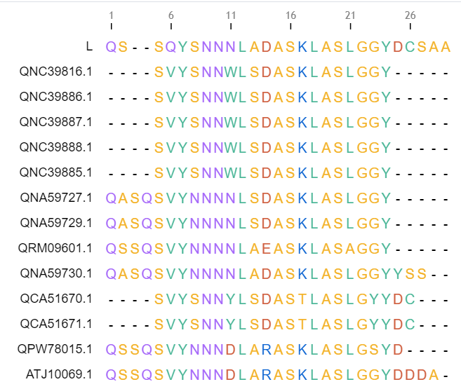
如果需要查看某个检索到的序列的出处,可以根据检索的CDR的序列编号,从任务输出的log文件中找到对应的专利名,
例如序列ATJ10081.1来自于US专利9493553(SEQ ID为39),并且US专利9670274、9890209等多个专利中也出现了该CDR片段,他们的比对情况包括同源性也展示在后面,如下图所示。
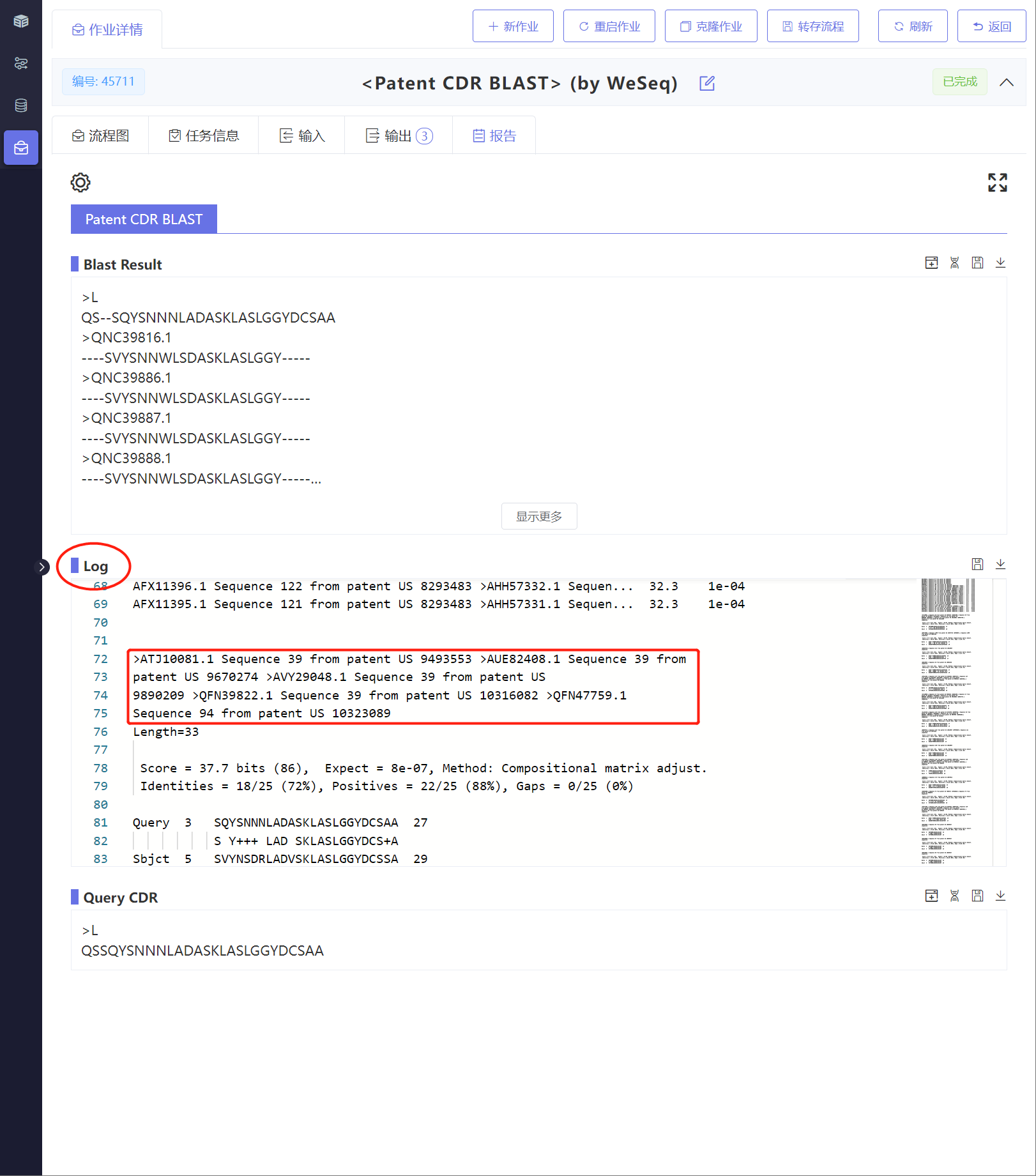
根据唯信团队经验,通常CDR的保护范围精确到具体序列,即差异一个以上氨基酸,即视为不在专利的保护范围之内,但不排除存在等同侵权的风险,仅供参考。
抗体序列文件, FASTA格式
指定序列比对数据库类型:抗体全长(full)或者抗体CDR区域 (cdr)。
CDR区域数据库为专利保护抗体数据库。
输出结果包括:
| 输出文件名称 | 说明 |
|---|---|
| align.fst | 序列比对结果文件 |
| blast.log | 序列比对日志文件 |
A module for sequence retrieval of antibody full-length or CDR region. When retrieving an antibody variable region from a patent, existing BLAST programs (such as NCBI BLAST) usually search the whole sequence, but for antibodies, the function mainly depends on the CDR, FR is relatively not important, and due to the generality of FR, FR of many different antibodies is the same or highly homologous. However, FR accounts for a higher proportion of sequences, resulting in a lot of sequences with similar FR but different CDR by BLAST in the variable region of antibodies. Moreover, in addition to protecting the complete sequence of the variable region during patent application, in many cases, the antibody CDR will also be protected separately to obtain a wider range of protection, so it is necessary to search for homologous sequences with CDR as the target in the process of antibody development. To this end, the Vixon team developed the program, which can retrieve the closest sequence to the target CDR from the existing patent library. Data updated: Dec 2024
For example, when inputting the complete sequence of antibody L for search, the returned CDR of the highly homologous sequences is shown in the image below.
If there is a need to check the source of a retrieved sequence, you can find the corresponding patent name based on the sequence number of the retrieved CDR from the log file output of the task. For example, sequence ATJ10081.1 is from US Patent 9493553 (SEQ ID 39), and the CDR fragment also appears in multiple patents such as US Patents 9670274, 9890209, etc., with their alignment details and homology shown as well, as depicted in the image below.
Based on the experience of the WeMol team, the protection range of CDRs is usually specified down to the specific sequence, meaning that a difference of one or more amino acids is considered outside the scope of patent protection. However, there may still be risks of equivalent infringement, so this information is for reference only.
Antibody sequence file in FASTA format.
Specifies the sequence alignment database type: antibody full-length (full) or antibody CDR region (cdr).
The CDR regional database is a patent protected antibody database.
The output includes:
| Output File Name | Description |
|---|---|
| align.fst | Sequence alignment result file |
| blast.log | Sequence alignment log file |

CIF2PDB模块是基于BioPython将mmCIF文件转换成PDB文件。
单独化合物CIF转换部分存在问题。
输入所需的 mmCIF 格式结构文件。
.cif 文件或其压缩包。.zip, .tar.gz, .tar.bz2, .tar.xz, .tar。convert_output.pdb 的 PDB 文件。convert_output.tar.gz 的压缩包,其中包含转换后的所有 PDB 文件。The CIF2PDB module is based on BioPython to convert mmCIF files into PDB files.
The structural file(s) in mmCIF format.
.cif files or compressed archives..zip, .tar.gz, .tar.bz2, and .tar.xz.convert_output.pdb.convert_output.tar.gz containing the converted PDB files.基于MIT(麻省理工学院)的Boltz-2算法的AF3 like结构预测模型。Boltz-2是一种开源深度学习模型,融合了模型架构、速度优化和数据处理方面的创新,在预测生物分子复合物的 3D结构方面达到了 AlphaFold3 级的准确度。Boltz-2 在一系列不同的基准测试中表现出与最先进的商业模型相当的性能,为结构生物学中可商业化使用的工具树立了新的标杆。

更新
相比于Boltz-1x,Boltz-2新增亲和力预测。
Boltz-2 是一个专为“生物分子交互”设计的 AI 大模型,它可以:
目前,最准确的亲和力预测方法是“自由能微扰(FEP)”,但它计算成本高,跑一次可能要几天。
相比之下:
Boltz-2 在多个实际药物研发场景中展现了优异性能:
虽然我们不展开技术细节,但 Boltz-2 之所以强大,主要靠以下三点:
Boltz-2 为药物研发、蛋白结构预测、AI 驱动分子设计提供了一个强大的通用平台:
Boltz-2 让 AI 第一次真正具备了“预测小分子是否好用”的能力,速度快、准确率高,开启新一代智能药物发现时代。
Q1:Boltz‑2 为什么不默认开启 Steering(结构引导)?
A:Steering 会让推理变慢约 2 倍,而且当前参数是在不使用 Steering 的情况下优化的。未来可能默认开启,但需重新调参。
Q2:Steering Potential 会不会让结构偏离真实构象?
A:Steering 的目的是将采样引导回“真实分布流形”,不会盲目收缩采样空间,但需要在“有效性”与“物理合理性”之间找到平衡。
Q3:结构相似性是按口袋还是全结构算的?会不会数据泄漏?
A:使用的是全结构相似性,这确实存在争议,但现实中药物研发常常面对有序列信息的靶点。我们已尽力控制信息泄漏风险。
Q4:Boltz‑2 的亲和力预测是回归还是分类?
A:两者都有,输出包括:
Q5:亲和力数据怎么处理?不准确怎么办?
A:主要训练 ∆Ki(同一实验内的相对值),因为原始 Ki/IC50 数据误差大。用 Cheng–Prusoff 公式统一 Ki 与 IC50。训练集只保留剂量-反应测量,删除噪声高/不可重复实验。
Q6:Boltz‑2 对结构准确性要求高吗?
A:是的,只训练了 ipTM ≥ 0.75 的结构。结构质量是亲和力预测成功的前提。
Q7:Boltz‑2 是否支持金属离子相关配体?
A:不支持。带金属离子的复合物在数据准备阶段已被过滤掉。
Q8:适用于哪些分子体系?
A:蛋白、小分子、RNA、DNA 等多模态复合物。对于大构象变化或柔性蛋白,性能会下降。
Q9:Boltz‑2 和 OpenFE、FEP+ 比如何?
A:在公开 benchmark 上性能优于 OpenFE,略低于商业级 FEP+,但速度优势巨大(~1000× 快)。
Q10:在 Recursion 内部数据集上效果好吗?
A:效果一般,说明模型仍对真实分布存在泛化问题。
Q11:能用于蛋白–蛋白亲和力预测吗?
A:还不支持,但开发中,预计未来几个月会发布 PPI affinity 模块。
Q12:能预测 ADME 或毒性吗?
A:某些毒性通路是结合驱动的,可以利用结构模型辅助预测。参考 BioEmu(Frank Noé)相关研究。
Q13:能预测药物耐药性吗?
A:我们也想知道,希望后续能验证。
Q14:Boltz‑2 可以与 MD 数据结合使用吗?
A:有讨论过,但还没有标准策略,未来可能探索“Boltz + MD”混合建模框架。
蛋白的序列文件,FASTA格式,支持多条序列。
注意:多蛋白复合物结构预测,其氨基酸序列输入格式如下:
>protein1
AASJ...
>protein2
AASJ...
>peptide
ASDF...
DNA核酸的序列文件,FASTA格式,支持多条序列。
RNA核酸分子的序列文件,FASTA格式,支持多条序列。
备注:当前24GB的GPU显存支持计算的残基/碱基数量在1000个左右。
文本文件包含小分子信息,TXT格式。支持SMILES或 CCD Code(化学组分词典编号)。如果使用SMILES格式,每行应包含一个小分子;如果使用CCD Code,每行可以包含一个或多个小分子,使用逗号分隔,并加上CCD前缀。示例如下:
CC(=O)OC1C[NH+]2CCC1CC2
CCD,ATP,HY3,P1L
CCD,MG
注意:不适用于配体蛋白或多肽的氨基酸序列格式输入。
包含翻译后修饰(PTM)信息的文本文件,TXT格式。每行放置一个PTM信息,每个PTM信息由三部分组成:
1,HY3,1 表示第一条序列的第一个残基,发生了类型为HY3(CCD编号,为3-羟基脯氨酸,为脯氨酸的羟基化)的PTM1,HY3,1
1,P1L,5
2,HY3,3
指定需要环化的序列的顺序编号,如1,2表示第一和第二条序列都进行首尾相连的环化。
共价键信息的文本文件,TXT格式。每行放置一个共价键信息,每个共价键信息包含两个原子信息,每个原子信息由三部分组成:
3,1,CA表示第三个实体(序列或小分子)中的第一个残基(或小分子)的CA原子1,1,CA;2,1,CA1,1,CA,第二个原子为2,1,CA1,1,CA;2,1,CA
1,1,CA;3,1,CHA
接触类型限制信息的文本文件,TXT格式。每行放置一个接触对(残基或小分子CCD中的标准原子名称)的信息,每个接触对信息由三部分组成:
1,25 表示第一个实体(序列)的第25个残基,2,CA表示第二个实体(小分子)中的CA原子。6.0,支持范围为4.0-20.0之间上述三部信息之间也用英文分号“;”进行分隔,例如:1,35;2,62;6.0表示第一条序列中的第35号残基,与第二条序列的第62号残基,靠近接触,且两者之间的最大距离为6埃。1,35;2,CA;6.0表示第一条序列中的第35号残基,与第二个实体(小分子)的CA原子,靠近接触,且两者之间的最大距离为6埃。
包含多个结合位点信息的文件内容示例如下:
1,35;2,62;6.0
1,48;2,CA;6.0
结合位点类型限制信息的文本文件,TXT格式。每行放置一个结合位点信息,每个结合位点信息由三部分组成:
1,25 表示第一条序列中的第25个残基;可以定义多个残基信息,由英文分号“;”进行分隔,如1,25;1,27;1,32;1,38表示第一条序列中的第25/27/32/38号残基形成结合位点6.0,支持范围为4.0-20.0之间上述三部信息之间也用英文分号“;”进行分隔,例如:2;1,55;1,62;1,91;1,92;1,99;1,110;6.0表示第二个实体(序列或小分子)作为Binder,与第一条序列的第55/62/91/92/99/110号残基所形成的结合位点进行结合。且两者之间的最大距离为6埃。
包含多个结合位点信息的文件内容示例如下:
2;1,55;1,62;1,91;1,92;1,99;1,110;6.0
3;1,25;1,27;1,32;1,38;8.0
指定结构建模时,使用的模板结构文件,PDB或CIF格式(推荐CIF格式,PDB格式缺失头信息时Boltz处理会报错),当前仅适用于蛋白序列。
在使用模板进行结构建模时,是否增加强制约束:
True:模板作为硬约束,预测的结构会被"强制"向模板结构靠拢,而非仅作为参考信息。通过在能量函数中引入约束势能(restraint potential)来实现。注意:此模式可能会引起部分结构的断裂。
False:模板仅作为参考信息,允许预测结构与模板结构之间存在较大偏离。默认为False。
在设置了Template参数时,如果只希望部分蛋白序列基于模板进行建模,可指定该参数,设置需要进行模板建模的蛋白序列顺序编号(同Modification参数中定义),支持多条蛋白序列,用英文逗号分隔。
例如:只希望第一条蛋白序列使用模版建模,该参数设置为1即可。如果希望第一条与第二条蛋白序列使用模版建模,该参数设置为1,2即可。
指定小分子顺序编号(定义见Bond参数),进行亲和力评估,格式为正整数,且只能指定1个小分子,如:3表示要进行亲和力评估的是顺序编号为3的小分子。模型会评估复合物体系中该小分子与其他部分的结合亲和力。
定义的残基区域信息。模块将输出区域中所有残基平均的pLDDT数值。一个残基区域由序列顺序编号与残基组合编号组成:
1:24,28,32-40 表示第一条序列中的第24/28/32至40号残基所组成的区域,因为是第一条序列,数值1可以省略,等同于24,28,32-40 ,该区域的所有残基的平均pLDDT值将输出到结果文件中。残基区域支持定义多个,每个残基区域之间用英文“;”分隔,例如:
1:24,28,32-40;2:15,23,50-60表示定义了两个区域,区域一为第一条序列的第24/28/32至40号残基,区域二为第二条序列的第15/23/50至60号残基。两个区域各自的残基平均pLDDT值,将输出到结果文件中。
随机数种子,用于控制预测过程中的随机性。
输出结构的格式,支持PDB或CIF格式,默认为PDB格式。
结构打分的结果文件名,默认为pred_scores_boltz.csv
亲和力打分的结果文件名,默认为pred_affinity_boltz.csv
批量预测模式采用阶梯式动态计费,根据预测结构数量分段计费,规则如下:
注意:
1.当前系统最多支持 1000 个结构的批量预测
2.一条fasta序列为一个结构
蛋白的序列文件,FASTA格式,支持多条序列。
每一条记录代表一个待预测的结构,每条记录的名称要唯一不能重复。一条记录中有多条链时,通过英文冒号(:)相连,文件内容示例如下:
>1
EVQLVESGGGVVQPGRSLRLS:NFMLTQPHSVSVL:ELFPQWHLPIKIAAIIAS
>2
YYCAKDRRDMGYFQHWGQGTLVTVSSQWYQQRPGSAPTTVIYEDNQRPSGTPPTFMIAVFLPIVVLIFKSILFL
表示有两个待预测的结构,第一条记录的名称为1,有三条蛋白链,用:进行分隔。第二条记录的名称为2,为单链。
DNA核酸的序列文件,FASTA格式,支持多条序列。
每一条序列记录代表一个待预测的结构,每条记录的名称要唯一不能重复(可与Protein参数中的记录名称一致,表示该记录的DNA序列与Protein序列归属于同一结构)。一条记录中有多条链时,通过英文冒号(:)相连,文件内容示例如下:
>dna
GACCTCT:CCTAGCT
>1
CCTAGCT
表示有两条记录,第一条的名称为dna,有两条DNA链,用:进行分隔,因为该名称不存在与Protein示例记录中,属于新结构。第二条的名称为1,有一条DNA链,因为该名称存在于Protein示例记录中,则表示同属一个结构(该结构同时包含Protein序列和该DNA序列)。
RNA核酸分子的序列文件,FASTA格式,支持多条序列。
每一条序列记录代表一个待预测的结构,每条记录的名称要唯一不能重复(可与DNA或Protein参数中的记录名称一致,表示该记录的RNA序列与上面的DNA序列或Protein序列归属于同一结构)。一条记录中有多条链时,通过英文冒号(:)相连,文件内容示例如下:
>1
AGCU
>rna
AGGCU:UGAUC
表示有两条记录,第一条的名称为1,为单链,因为该名称存在于DNA及Protein示例记录中,表示同属一个结构(该结构同时包含了Protein序列、DNA序列及该RNA序列)。第二条的名称为rna,有两条RNA链,用:进行分隔,因为该名称不存在于DNA或Protein示例记录中,属于新结构。
文本文件包含小分子信息,TXT格式。支持SMILES或 CCD Code(化学组分词典编号)。如果使用SMILES格式,每行应包含一个小分子;如果使用CCD Code,每行可以包含一个或多个小分子,使用逗号分隔。
每行代表一个待预测的结构,每行可放置多个ligand,且以唯一不重复的名称开头(该名称可与上述RNA,DNA或Protein参数中的记录名称一致,表示该行的所有ligands,与上述的RNA或DNA或Protein序列归属于同一结构),名称与所有ligands都以英文冒号(:)分隔。文件内容示例如下:
1:CC(=O)OC1C[NH+]2CCC1CC2:CCD,ATP,HY3
lig:CC1CC(CN2NC[N+](=C3CCC(OC(F)(F)F)CC3)C2=O)CC(C)C1OC(C)(C)C(=O)[O-]
表示有两条记录,第一条的名称为1,有三个ligand(一个SMILES,两个CCD codes),因为该名称存在于上述的RNA或DNA或Protein示例记录中,表示同属一个结构。第二条的名称为lig,有一个ligand(为SMILES),因为该名称不存在上述的RNA或DNA或Protein示例记录中,属于新结构。
注意:
1.不适用于配体蛋白或多肽的氨基酸序列格式输入。
2.在预测每个结构的序列数量相同的情况下,可为所有待预测结构设置相同的小分子信息,设置方式为输入一行小分子信息(可多个),且不设置结构名称,如CC(=O)OC1C[NH+]2CCC1CC2:CCD,ATP,表示为所有结构都加入小分子CC(=O)OC1C[NH+]2CCC1CC2与ATP。
包含翻译后修饰(PTM)信息的文本文件,TXT格式。每个PTM的信息与Single模式中一致(参考Single模式中的定义)。
每行定义一个结构的所有PTM信息,且以唯一名称开头(该名称必须存在于前述的Protein或DNA或RNA记录中),都以英文冒号(:)分隔。文件内容示例如下:
1:1,HY3,1:1,P1L,5:2,HY3,3
2:1,HY3,1:2,HY3,3
表示前述名称为1的结构中(Protein或DNA或RNA),有三个PTM。名称为2的结构中,有两个PTM。
注意:在预测每个结构的序列数量相同的情况下,可为所有待预测结构设置相同的PTM信息,设置方式为输入一行PTM信息,且不设置结构名称,如:1,HY3,1:1,P1L,5:2,HY3,3表示这些PTM信息将应用到所有结构。
包含需要环化的序列顺序编号的文本文件,TXT格式。每行定义一个结构的所有环化序列信息,且以唯一名称开头(该名称必须存在于前述的Protein或DNA或RNA记录中),都以英文冒号(:)分隔。文件内容示例如下:
complexA:2
complexB:2,3
表示前述名称为complexA的结构中(Protein或DNA或RNA),顺序编号为2的序列进行首尾相连的环化。名称为complexB的结构中,顺序编号为2和3的序列都进行首尾相连的环化。
注意:在预测每个结构的序列数量相同的情况下,可为所有待预测结构设置相同的环化信息,设置方式为输入一行环化信息,且不设置结构名称,如:2,表示为所有结构设置环化序列编号为2。
共价键信息的文本文件,TXT格式。每个共价键的信息与Single模式中一致(参考Single模式中的定义)。
Batch模式下,每行定义一个结构的所有共价键,且以唯一名称开头(该名称必须存在于前述的Protein或DNA或RNA记录中),都以英文冒号(:)分隔。文件内容示例如下:
1:1,1,CA;2,1,CA:1,1,CA;3,1,CHA
2:1,1,CA;3,1,CHA
表示前述名称为1的结构中(Protein或DNA或RNA),有两个共价键。名称为2的结构中,有一个共价键。
注意:在预测每个结构的序列数量相同的情况下,可为所有待预测结构设置相同的共价键信息,设置方式为输入一行共价键信息,且不设置结构名称,如:1,1,CA;3,1,CHA表示该共价键信息将应用到所有结构。
接触类型限制信息的文本文件,TXT格式。每个接触信息的定义与Single模式中一致(参考Single模式中的定义)。
Batch模式下,每行定义一个结构的所有接触信息,且以唯一名称开头(该名称必须存在于前述的Protein或DNA或RNA记录中),都以英文冒号(:)分隔。文件内容示例如下:
1:1,35;2,62;6.0
2:1,48;2,CA;6.0:1,35;2,62;6.0
表示前述名称为1的结构中(Protein或DNA或RNA),有一个接触限制。名称为2的结构中,有两个接触限制。
注意:在预测每个结构的序列数量相同的情况下,可为所有待预测结构设置相同的接触信息,设置方式为输入一行接触信息,且不设置结构名称,如:1,35;2,62;6.0表示该Contact信息将被应用到所有结构。
结合位点类型限制信息的文本文件,TXT格式。每个结合位点信息的定义与Single模式中一致(参考Single模式中的定义)。
Batch模式下,每行定义一个结构的所有结合位点限制信息,且以唯一名称开头(该名称必须存在于前述的Protein或DNA或RNA记录中),都以英文冒号(:)分隔。文件内容示例如下:
1:2;1,55;1,62;1,91;1,92;1,99;1,110;6.0
2:1;2,15;2,17;2,18;2,56;6.0:1;3,76;3,78;3,96;8.0
表示前述名称为1的结构中(Protein或DNA或RNA),有一个结合位点限制。名称为2的结构中,有两个结合位点限制。
注意:在预测每个结构的序列数量相同的情况下,可为所有待预测结构设置相同的限制信息,设置方式为输入一行限制信息,且不设置结构名称。如:2;1,55;1,62;1,91;1,92;1,99;1,110;6.0表示该pocket信息将被应用到所有结构。
指定小分子顺序编号(定义见Bond参数),进行亲和力评估,每个亲和力信息的定义与Single模式一致。
Batch模式下,每行定义一个亲和力信息,且以唯一名称开头(该名称必须存在于前述的Protein或DNA或RNA记录中),都以英文冒号(:)分隔。文件内容示例如下:
1:4
2:5
表示前述名称为1的结构中(Protein或DNA或RNA),有亲和力计算,其小分子Binder的顺序编号为4。名称为2的结构中,有亲和力计算,其小分子Binder的顺序编号为5。
注意:
1.Batch模式中如果设置该参数Affinity,则需要批量预测的每个结构中都有设置Affinity信息,否则会提示错误。
2.小分子 Binder 排序仅依赖 Protein、DNA、RNA 参数的序列顺序与数量,Ligand 不参与排序。**
3.在预测每个结构的序列数量相同的情况下,可为所有待预测结构设置相同的亲和力信息,设置方式为输入小分子的顺序编号4,且不设置结构名称
指定结构建模时,使用的模板结构文件(同Single模式),当前仅适用于蛋白序列。
输出结构的格式,支持PDB或CIF格式,默认为PDB格式。
随机数种子,用于控制预测过程中的随机性。
虚拟筛选模式中,可一次性提交多个小分子,每个小分子会单独与蛋白/核酸体系计算亲和力。当前一次运行支持最大100个小分子。
蛋白的序列文件,FASTA格式,支持多条序列。(同Single模式)
DNA核酸的序列文件,FASTA格式,支持多条序列。(同Single模式)
RNA核酸分子的序列文件,FASTA格式,支持多条序列。(同Single模式)
备注:当前24GB的GPU显存支持计算的残基/碱基数量在1000个左右。
文本文件包含小分子信息,TXT格式。支持SMILES或 CCD Code(化学组分词典编号)。如果使用SMILES格式,每行应包含一个小分子;如果使用CCD Code,每行可以包含一个或多个小分子,使用逗号分隔,并加上CCD前缀。示例如下:
CC(=O)OC1C[NH+]2CCC1CC2
CCD,ATP,HY3,P1L
CCD,MG
包含翻译后修饰(PTM)信息的文本文件,TXT格式。(同Single模式)
指定需要环化的序列的顺序编号,如1,2表示第一和第二条序列都进行首尾相连的环化。(同Single模式)
共价键信息的文本文件,TXT格式。(同Single模式,但共价键中小分子不能参与)
结合位点类型限制信息的文本文件,TXT格式。(同Single模式)
亲和力打分的结果文件名,默认为pred_affinity_boltz.csv
输出结果文件为排名前5的复合物结构rank_1-5.cif,pred_scores_boltz.csv,pred_affinity_boltz.csv(如果指定了Affinity参数)和可视化交互式工具PAE Viewer生成的boltz_report.html和pae_report_Model_1-5.html。
pred_scores_boltz.csv中包含信息如下:
| 字段名称 | 说明 |
|---|---|
| Name | 复合物结构名称 |
| Confidence_Score | 对预测结构的质量排序的指标分数,数值在0~1.0之间,越大表示预测结构的质量越高。 该分数综合考虑了两个指标:iptm(单体时为pTM), complex_plddt, 计算公式为: Confidence_Score = 0.8 × complex_plddt + 0.2 × ipTM |
| pTM | 对结构预测得到的TM score,衡量预测结构整体准确性,越大表示越准确,该分数大于0.5时,表示结构整体折叠可能与真实结构相似 |
| ipTM | 对结构中的相互作用界面预测得到的TM score,当预测结构为复合物时才有该评价指标,衡量复合物中各个亚基之间相对位置的预测准确性,越大表示越准确。 大于0.8表示高质量预测, 小于0.6表示预测可能失败, 0.6-0.8为灰色地带,预测正确与否不确定 |
| ipSAE | 基于pAE(predicted Aligned Errors)矩阵计算得到的相互作用界面评价分数,取值范围是0到1,值越大,表示预测的蛋白-蛋白相互作用界面越可靠。 ipSAE > 0.7 表明相互作用界面预测质量高,结构可信。 ipSAE < 0.1: 表明预测中几乎不存在可信互作界面,可排除假阳性相互作用。 |
| Complex_pLDDT | 对复合物预测得到的平均pLDDT score,值范围是0-1.0,该值越大说明预测的结构越可靠。低于0.7被认为可靠性较低,低于0.5基本认为是可信度非常低,为无序预测 |
| Complex_ipLDDT | 将复合物中相互作用界面的权重提升后,预测得到的pLDDT score,值范围是0-1.0,该值越大说明预测的结构越可靠 |
| complex_pDE | 复合物中所有残基对之间的平均预测距离误差,是评估复合物结构预测质量的指标,越低越好。典型数值范围:高质量区域:< 2 Å,中等质量区域:2-5 Å,低质量/柔性区域:> 5 Å |
| complex_ipDE | 复合物界面区域残基对的平均预测距离误差,越低越好,专门反映界面相互作用的预测可靠性,阈值范围同上。 |
| pLDDT_domain | 当设置Domain参数时,预测得到的区域残基的平均pLDDT数值,多个区域时,数值用英文分号";"分隔 |
| Avg_pAE | 平均pae分数,pae是预测对齐误差,是残基对水平的置信度指标,用来衡量任意两个残基之间相对空间位置的预测可信度。 数值<5,表示残基对之间相对位置预测非常可靠,通常位于同一结构域内; 数值在5–10,表示预测较为准确,可能为柔性环区或轻微构象差异区域; 数值在10–20,表示相对位置不确定性较高,常见于结构域间连接区或柔性区域; 数值> 20,表示预测不可靠,可能为无序区域、错误折叠,或复合物界面不稳定。 |
| Min_pAE | 所有pae分数中的最小值 |
| Avg_iPAE | 结构中相互作用界面的平均pae分数 |
| Min_iPAE | 结构中相互作用界面pae分数中的最小值 |
| Avg_Ligand_pAE | ligand存在时,与ligand相关的pAE分数的平均值。 |
| Min_Ligand_pAE | ligand存在时,与ligand相关的pAE分数的最小值。 |
| pDockQ2_链名 | 该链的预测对接评分(pDock2),用于评估该链在复合物界面中的结合可靠性 |
| pDockQ2_Avg | 链之间的平均预测对接评分,用于整体评估复合物界面质量 |
| pDockQ2 范围 | 结构质量评估 |
|---|---|
| < 0.23 | 不正确(Incorrect) |
| 0.23 – 0.49 | 可接受(Acceptable) |
| 0.49 – 0.80 | 中等质量(Medium) |
| > 0.80 | 高质量(High quality) |
pred_affinity_boltz.csv中包含信息如下:
| 字段名称 | 说明 |
|---|---|
| Pred_Affinity(log(IC50)) | 预测的复合物中小分子与其他部分结合的亲和力数值,为IC50的对数值,即log(IC50),其中IC50的单位为μM,数值越低表示亲和力越强。 |
| Pred_Prob | 概率值,判断小分子是真正Binder的可能性,数值在0-1之间,越大表示小分子是Binder的可能性越大 |
输出final_results.tar.gz、pred_scores_boltz.csv以及pred_affinity_boltz.csv(如果指定了Affinity参数)
final_results.tar.gz文件为Batch模式下生成一个所有预测结果的打包文件,包含预测结构PDB文件、打分CSV文件。
pred_scores_boltz.csv以及pred_affinity_boltz.csv。(同Single模式)
输出pred_affinity_boltz.csv文件为亲和力预测结果,包含如下信息:
| 字段名称 | 说明 |
|---|---|
| ID | 小分子顺序,从1开始 |
| Ligand | 小分子的SMILES或CCD代码 |
| Pred_Affinity(log(IC50)) | 预测的复合物中小分子与其他部分结合的亲和力数值,为IC50的对数值,即log(IC50),其中IC50的单位为μM,数值越低表示亲和力越强。 |
| Pred_Prob | 概率值,判断小分子是真正Binder的可能性,数值在0-1之间,越大表示小分子是Binder的可能性越大 |
final_results.tar.gz文件为所有预测结果的打包文件,包含预测结构PDB文件、打分CSV文件。
Developed based on the Boltz-2 model, Boltz-2 is an open-source deep learning model that integrates innovations in model architecture, speed optimization, and data processing. It achieves AlphaFold3-level accuracy in predicting the 3D structures of biomolecular complexes. Boltz-2 demonstrates performance comparable to state-of-the-art commercial models across a range of benchmarks, setting a new standard for commercially usable tools in structural biology.
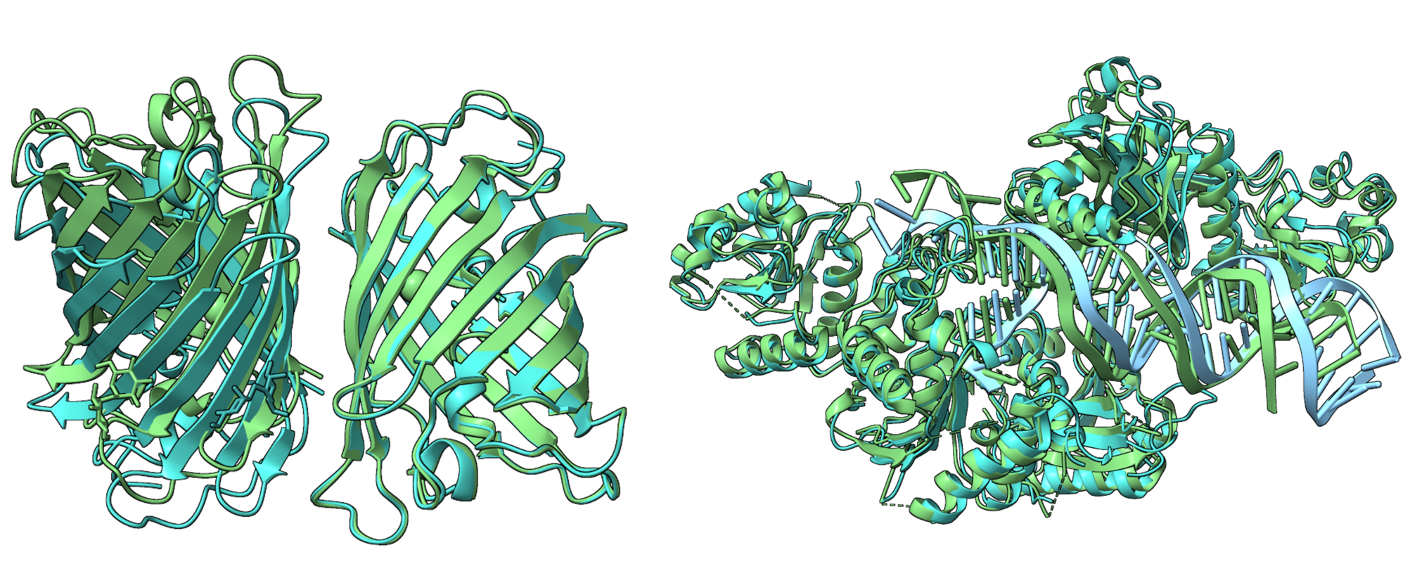
Updates
Compared to Boltz-1x, Boltz-2 has added the capability of affinity prediction.
Boltz-2 is an AI model specifically designed for “biomolecular interactions”. It can:
Currently, the most accurate method for affinity prediction is Free Energy Perturbation (FEP), but it is computationally expensive and can take days to complete a single calculation.
In comparison:
Most importantly, Boltz-2 is open-source, meaning both researchers and pharmaceutical companies can use it for free!
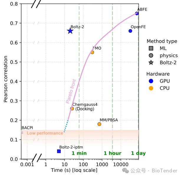
Boltz-2 presents a strong accuracy/speed trade-off for affinity prediction.
Boltz-2 has demonstrated outstanding performance in various real-world drug discovery scenarios:
Drug Optimization
In test datasets, Boltz-2 can accurately determine which small molecule binds more strongly, achieving results close to FEP but 1000 times faster.
Virtual Screening
When faced with hundreds of thousands of small molecules, Boltz-2 quickly identifies potential active compounds. For example, in the TYK2 target test, 8 out of the top 10 molecules selected by Boltz-2 were later validated as effective in simulations.
Enhanced Structure Prediction
Compared to its predecessor, Boltz-2 performs better on complex structures such as RNA and antibodies. It can also customize predictions based on experimental conditions.
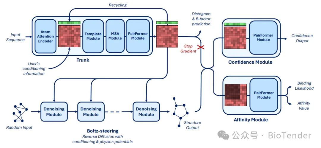
Boltz-2 model architecture diagram
While we won’t dive into the technical details, Boltz-2’s strength lies in three key aspects:
Smarter Data Curation
The team carefully selected high-quality data from massive public databases and removed noise, resulting in a more reliable model.
Integration with Generative Models
Boltz-2 not only evaluates interactions but also works with molecular generative models to design new small molecules, significantly expanding the chemical space.
Greater Customizability
Researchers can specify conditions for structure predictions, such as incorporating NMR experimental data or focusing on specific binding sites of interest. The model adapts flexibly.
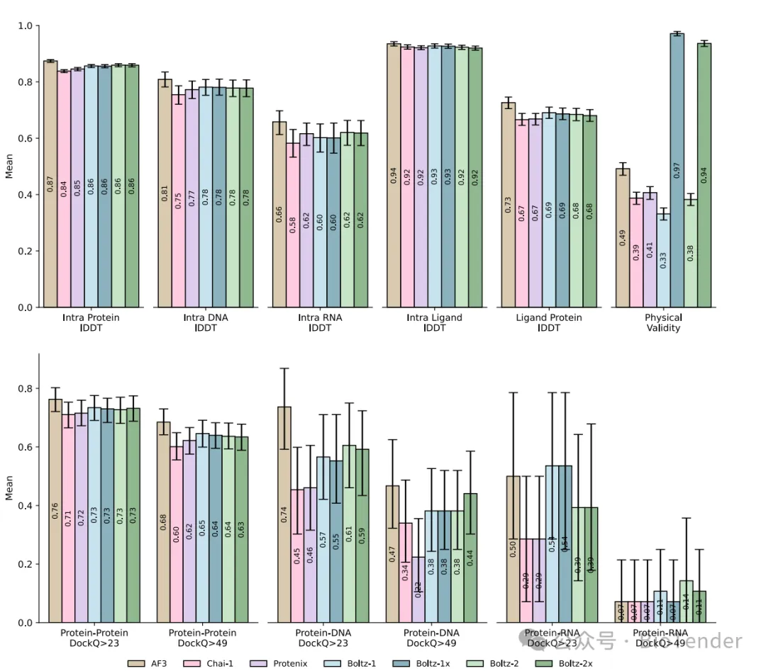
Evaluation of the performance of Boltz-2 against existing co-folding models on a diverse set of unseen complexes
Boltz-2 provides a powerful, general-purpose platform for drug discovery, protein structure prediction, and AI-driven molecular design:
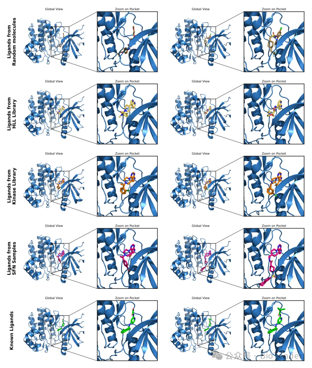
Boltz-2 empowers AI to truly predict the effectiveness of small molecules for the first time, combining speed and accuracy to usher in a new era of intelligent drug discovery.
Q1: Why doesn’t Boltz-2 enable Steering (structural guidance) by default?
A: Steering slows inference by about 2x, and the current parameters are optimized without Steering. It may be enabled by default in the future, but parameter tuning will be required.
Q2: Does Steering Potential cause structures to deviate from their true conformations?
A: Steering aims to guide sampling back to the “manifold of true distributions” without blindly shrinking the sampling space. However, it requires a balance between “effectiveness” and “physical plausibility.”
Q3: Is structural similarity calculated based on the pocket or the entire structure? Could there be data leakage?
A: Structural similarity is calculated using the entire structure, which is indeed a controversial approach. However, in real-world drug discovery, target sequence information is often available. Efforts have been made to minimize the risk of information leakage.
Q4: Is Boltz-2’s affinity prediction regression-based or classification-based?
A: Both. The output includes:
Q5: How is affinity data processed? What happens if it’s inaccurate?
A: The model primarily trains on ∆Ki (relative values within the same experiment) due to large errors in raw Ki/IC50 data. Ki and IC50 values are unified using the Cheng–Prusoff equation. The training set excludes high-noise or non-reproducible experiments, focusing on dose-response measurements.
Q6: Does Boltz-2 require high structural accuracy?
A: Yes, it only trains on structures with ipTM ≥ 0.75. Structural quality is essential for successful affinity prediction.
Q7: Does Boltz-2 support ligands with metal ions?
A: No, complexes containing metal ions are filtered out during data preparation.
Q8: What molecular systems is Boltz-2 suitable for?
A: Protein, small molecules, RNA, DNA, and other multi-modal complexes. Performance decreases for systems with large conformational changes or flexible proteins.
Q9: How does Boltz-2 compare to OpenFE and FEP+?
A: It outperforms OpenFE on public benchmarks but slightly underperforms compared to the commercial-grade FEP+. However, Boltz-2 has a significant speed advantage (~1000× faster).
Q10: Does Boltz-2 perform well on Recursion’s internal datasets?
A: Performance is moderate, indicating the model still struggles with generalization to real-world distributions.
Q11: Can Boltz-2 predict protein–protein affinity?
A: Not yet, but development is underway. A PPI affinity module is expected in the coming months.
Q12: Can Boltz-2 predict ADME or toxicity?
A: Certain toxicity pathways are binding-driven, and structural models can assist in prediction. Related studies include BioEmu by Frank Noé.
Q13: Can Boltz-2 predict drug resistance?
A: We hope to explore this in future validations.
Q14: Can Boltz-2 be used with MD data?
A: There have been discussions, but no standard strategy exists yet. A future direction may involve exploring a “Boltz + MD” hybrid modeling framework.
The sequence file of proteins in FASTA format, supporting multiple sequences.
Note: For multi-protein complex structure prediction, the amino acid sequence input format is as follows:
>protein1
AASJ...
>protein2
AASJ...
>peptide
ASDF...
The sequence file of DNA nucleic acids in FASTA format, supporting multiple sequences.
The sequence file of RNA nucleic acid molecules in FASTA format, supporting multiple sequences.
A text file containing small molecule information in TXT format. It supports SMILES or CCD Code (Chemical Component Dictionary number). If using the SMILES format, each line should contain one small molecule; if using the CCD Code, each line can contain one or more small molecules, separated by commas and prefixed with CCD. An example is as follows:
CC(=O)OC1C[NH+]2CCC1CC2
CCD,ATP,HY3,P1L
CCD,MG
Note: Not applicable for amino acid sequence format input of ligand proteins or polypeptides.
A text file containing post-translational modification (PTM) information in TXT format. Each line contains one PTM information entry, consisting of three parts:
1,HY3,1 indicates that the first residue of the first sequence undergoes a PTM of type HY3 (CCD number, which is 3-hydroxyproline, a hydroxylation of proline).Note:
An example of a file containing multiple PTM information entries is as follows:
1,HY3,1
1,P1L,5
2,HY3,3
Specify the serial numbers of the sequences to be cyclized; for example, 1,2 indicates that both the first and the second sequences undergo head-to-tail cyclization.
A text file containing covalent bond information in TXT format. Each line contains one covalent bond information entry, and each entry includes two atom information entries, each consisting of three parts:
The three parts are separated by commas. For example, 3,1,CA indicates the CA atom of the first residue (or small molecule) in the third entity (sequence or small molecule).
A covalent bond consists of two atom information entries, separated by a semicolon, such as 1,1,CA;2,1,CA, indicating a covalent bond composed of two atoms: the first atom is 1,1,CA, and the second atom is 2,1,CA.
An example of a file containing multiple covalent bond information entries is as follows:
1,1,CA;2,1,CA
1,1,CA;3,1,CHA
A text file in TXT format that contains restricted information about contact types. Each line holds the information for one contact pair (residue or standard atom name in a small-molecule CCD), consisting of three parts:
1,25 denotes the 25th residue in the first entity (sequence), and 2,CA denotes the CA atom in the second entity (small molecule).6.0. Supported range is 4.0–20.0.These three pieces of information are separated by a semicolon “;”.
Example: 1,35;2,62;6.0 means that residue 35 of the first sequence and residue 62 of the second sequence are in close contact, with a maximum distance of 6 Å.
1,35;2,CA;6.0 means that residue 35 of the first sequence and the CA atom of the second entity (small molecule) are in close contact, with a maximum distance of 6 Å.
A file containing multiple binding-site entries would look like:
1,35;2,62;6.0
1,48;2,CA;6.0
A text file with pocket type restriction information, in TXT format. Each line contains the information of one pocket, which is composed of three parts:
6.The above three pieces of information are also separated by an English semicolon “;”. For example: 2;1,55;1,62;1,91;1,92;1,99;1,110 indicates that the second entity (sequence or small molecule) as a Binder, binds to the pocket formed by the 55th, 62nd, 91st, 92nd, 99th, and 110th residues in the first sequence. The maximum distance between the Binder and Pocket residues is 6 angstroms.
An example of a file content containing multiple pockets information is as follows:
2;1,55;1,62;1,91;1,92;1,99;1,110;6.0
3;1,25;1,27;1,32;1,38;8.0
The template structure file used in designated - structure modeling, in PDB or CIF format. Currently, it’s only applicable to protein sequences.
When performing structure modeling with a template, you can choose whether to apply forced constraints:
True:The template is treated as a hard constraint, meaning the predicted structure will be forced to align closely with the template rather than using it only as a reference.This is achieved by introducing restraint potentials into the energy function.
Note: This mode may cause structural breaks in some regions.
False:The template is used only as reference information, allowing the predicted structure to deviate significantly from the template if necessary.Default: False
When the Template parameter is set, to perform template - based modeling for certain part of the protein sequence, specify the order number(s) (as defined in the Modification parameter) of the target protein sequence(s). Multiple sequences are separated by commas.
Examples: Set to 1 to model the first protein sequence; set to 1,2 to model the first and second sequences.
Specify the serial number of the small molecule (defined in the Bond parameter) for affinity evaluation. The format must be a positive integer, and only one small molecule can be specified. For example, 3 indicates that the small molecule with the serial number 3 is to be evaluated for affinity. The model will assess the binding affinity of this small molecule with other components in the complex system.
The defined residue region information. The module will output the average pLDDT value of all residues in the region. A residue region is composed of sequence order numbers and residue combination numbers:
Sequence order numbers (as defined in the Modification parameter), the value 1 can be omitted (i.e., defaulting to 1).
Residue combination numbers, using residue position numbers, with multiple residues separated by commas and specified residue ranges indicated by hyphen symbols. For example, “3,10,24-30” indicates the 3rd, 10th, and 24th to 30th residues on the target sequence.
For example: 1:24,28,32-40 indicates the region composed of the 24th, 28th, and 32nd to 40th residues in the first sequence. Since it is the first sequence, the number 1 can be omitted, equivalent to 24,28,32-40. The average pLDDT value of all residues in this region will be output to the result file.
Multiple residue regions are supported, with each residue region separated by an English semicolon “;”. For example: 1:24,28,32-40;2:15,23,50-60 defines two regions. Region one consists of the 24th, 28th, and 32nd to 40th residues in the first sequence, and region two consists of the 15th, 23rd, and 50th to 60th residues in the second sequence. The average pLDDT values of the residues in each of the two regions will be output to the result file.
Random seed used to control the randomness in the prediction process.
The output structure format supports PDB or CIF, with PDB format as the default.
The filename for the structure scoring results, defaulting to “pred_scores_boltz.csv”.
The filename for the affinity scoring results, defaulting to “pred_affinity_boltz.csv”.
The batch prediction mode adopts a tiered, dynamic pricing model, where computational cost is charged based on the number of predicted structures:
Notes:
1. The system currently supports up to 1000 structures in a single batch prediction.
2. One FASTA sequence is counted as one structure.
The protein sequence file in FASTA format, supporting multiple sequences. Each record represents a structure to be predicted, and each record name must be unique. If a record contains multiple chains, they should be connected by a colon (:). Example content:
>1
EVQLVESGGGVVQPGRSLRLS:NFMLTQPHSVSVL:ELFPQWHLPIKIAAIIAS
>2
YYCAKDRRDMGYFQHWGQGTLVTVSSQWYQQRPGSAPTTVIYEDNQRPSGTPPTFMIAVFLPIVVLIFKSILFL
This indicates two structures to be predicted, with the first record named 1 containing three protein chains separated by colons. The second record is named 2 and contains a single chain.
The DNA sequence file in FASTA format, supporting multiple sequences. Each sequence record represents a structure to be predicted, and each record name must be unique. (It can match the record names in the Protein parameter, indicating that the DNA sequence belongs to the same structure as the Protein sequence.) If a record contains multiple chains, they should be connected by a colon (:). Example content:
>dna
GACCTCT:CCTAGCT
>1
CCTAGCT
This indicates two records, with the first named dna containing two DNA chains separated by a colon. Since this name does not appear in the Protein example records, it represents a new structure. The second record is named 1, containing one DNA chain, and since this name exists in the Protein example records, it indicates that they belong to the same structure (which contains both Protein and DNA sequences).
The RNA sequence file in FASTA format, supporting multiple sequences. Each sequence record represents a structure to be predicted, and each record name must be unique. (It can match the record names in the DNA or Protein parameters, indicating that the RNA sequence belongs to the same structure.) If a record contains multiple chains, they should be connected by a colon (:). Example content:
>1
AGCU
>rna
AGGCU:UGAUC
This indicates two records, with the first named 1, which is a single chain. Since this name exists in the DNA and Protein example records, it indicates that they belong to the same structure (which includes Protein, DNA, and this RNA sequence). The second record is named rna, containing two RNA chains separated by a colon. Since this name does not appear in the DNA or Protein example records, it represents a new structure.
A text file containing information on small molecules in TXT format. It supports either SMILES or CCD Code. If using SMILES format, each line should contain one small molecule; if using CCD Code, each line can contain one or more small molecules, separated by commas. Each line represents a structure to be predicted, and each line must start with a unique name (this name can match those in the RNA, DNA, or Protein parameters, indicating that all ligands in that line belong to the same structure). The name and all ligands are separated by a colon (:). Example content:
1:CC(=O)OC1C[NH+]2CCC1CC2:CCD,ATP,HY3
lig:CC1CC(CN2NC[N+](=C3CCC(OC(F)(F)F)CC3)C2=O)CC(C)C1OC(C)(C)C(=O)[O-]
This indicates two records, with the first named 1, containing three ligands (one SMILES and two CCD codes). Since this name exists in the RNA, DNA, or Protein example records, it indicates that they belong to the same structure. The second record is named lig, containing one ligand (in SMILES format). Since this name does not appear in the RNA, DNA, or Protein example records, it represents a new structure.
Note:
1.In Batch mode, if the Affinity parameter is set, each structure in the batch must have Affinity information; otherwise, an error will be reported.
2.The sorting of small-molecule binders depends solely on the sequence order and quantity of the Protein, DNA, and RNA parameters; the ligand itself does not participate in the sorting.
3.You can assign the same ligand information to all target structures by providing a single line of ligand data (multiple ligands are allowed) without specifying structure names. For example:CC(=O)OC1C[NH+]2CCC1CC2:CCD,ATP
This indicates that all structures will include the ligands CC(=O)OC1C[NH+]2CCC1CC2 and ATP.
A text file containing post-translational modification (PTM) information in TXT format. Each PTM entry is consistent with that in Single mode (refer to the definitions in Single mode). Each line defines all PTM information for a structure, starting with a unique name (this name must exist in the previously defined Protein, DNA, or RNA records), separated by colons (:). Example content:
1:1,HY3,1:1,P1L,5:2,HY3,3
2:1,HY3,1:2,HY3,3
This indicates that the structure named 1 (Protein, DNA, or RNA) has three PTMs, while the structure named 2 has two PTMs.
Note: When the sequence count for each structure to be predicted is the same, you can set identical PTM information for all structures by entering a single line of PTM information without specifying a structure name. For example: 1,HY3,1:1,P1L,5:2,HY3,3 indicates that these PTM information will be applied to all structures.
A plain-text file (TXT) that lists the serial numbers of the sequences to be cyclized.
Each line defines the cyclization information for one structure and must start with the unique name of that structure (exactly as given in the preceding Protein / DNA / RNA records).
The name and the sequence numbers are separated by a colon (:).
Example file content:
complexA:2
complexB:2,3
In the structure named complexA, the 2nd sequence will be cyclized head-to-tail.
In the structure named complexB, both the 2nd and 3rd sequences will be cyclized head-to-tail.
Note: When the sequence count for each structure to be predicted is the same, you can set identical cyclization information for all structures by entering a single line of cyclization information without specifying a structure name. For example: 2 indicates that cyclization sequence index 2 will be set for all structures.
A text file containing covalent bond information in TXT format. Each covalent bond entry is consistent with that in Single mode (refer to the definitions in Single mode). In Batch mode, each line defines all covalent bonds for a structure, starting with a unique name (this name must exist in the previously defined Protein, DNA, or RNA records), separated by colons (:). Example content:
1:1,1,CA;2,1,CA:1,1,CA;3,1,CHA
2:1,1,CA;3,1,CHA
This indicates that the structure named 1 (Protein, DNA, or RNA) has two covalent bonds, while the structure named 2 has one covalent bond.
Note: When the sequence count for each structure to be predicted is the same, you can set identical covalent bond information for all structures by entering a single line of covalent bond information without specifying a structure name. For example: 1,1,CA;3,1,CHA indicates that this covalent bond information will be applied to all structures.
A text file in TXT format containing contact type restraint information. The definition of each contact restraint is consistent with that in Single mode (refer to the definition in Single mode).
In Batch mode, each line defines all contact restraints for one structure, starting with a unique name (which must exist in the aforementioned Protein, DNA, or RNA records), with fields separated by English colons (:). An example of the file content is as follows:
1:1,35;2,62;6.0
2:1,48;2,CA;6.0:1,35;2,62;6.0
This indicates that in the structure named 1 (Protein, DNA, or RNA mentioned above), there is one contact restraint. In the structure named 2, there are two contact restraints.
Note: When the sequence count for each structure to be predicted is the same, you can set identical contact information for all structures by entering a single line of contact information without specifying a structure name. For example: 1,35;2,62;6.0 indicates that this Contact information will be applied to all structures.
A text file containing pockets information in TXT format. Each pocket is consistent with that in Single mode (refer to the definitions in Single mode). In Batch mode, each line defines all pockets for a structure, starting with a unique name (this name must exist in the previously defined Protein, DNA, or RNA records), separated by colons (:). Example content:
1:2;1,55;1,62;1,91;1,92;1,99;1,110
2:1;2,15;2,17;2,18;2,56:1;3,76;3,78;3,96
This indicates that the structure named 1 (Protein, DNA, or RNA) has one pocket, while the structure named 2 has two pockets.
Note: When the number of sequences predicted for each structure is the same, you can assign the same constraint information to all target structures. To do this, provide a single line of constraint information without specifying structure names.
Specify the ligand index (as defined in the Bond parameter) to perform affinity evaluation. The definition of each affinity entry is consistent with the Single mode.
In Batch mode, each line defines one affinity entry and must start with a unique name (which must exist in the previously defined Protein, DNA, or RNA records), separated by a colon (:). An example is shown below:
1:4
2:5
This indicates that:
1 (Protein/DNA/RNA), affinity calculation is performed with ligand index 4.2, affinity calculation is performed with ligand index 5.Note:
4, without specifying a structure name. This indicates that affinity calculation will be performed for all structures, with the small molecule Binder’s sequential index being 4.The template structure file used in designated - structure modeling (Same as Single mode.), it’s only applicable to protein sequences.
When performing structure modeling with a template, you can choose whether to apply forced constraints (Same as Single mode.)
The output structure format supports PDB or CIF, with PDB format as the default.
Random seed used to control the randomness in the prediction process.
In virtual screening mode, you may submit multiple small molecules in one job. Each molecule will be docked independently against the protein/nucleic-acid system to compute its binding affinity. A single run supports up to 100 small molecules.
Protein sequence file in FASTA format; multiple sequences are allowed. (Same as Single mode.)
DNA sequence file in FASTA format; multiple sequences are allowed. (Same as Single mode.)
RNA sequence file in FASTA format; multiple sequences are allowed. (Same as Single mode.)
Note: With a 24 GB GPU, the current implementation accommodates ≈1,000 residues / bases.
Plain-text file containing small-molecule information (TXT format).
Supported formats:
CCD.Example:
CC(=O)OC1C[NH+]2CCC1CC2
CCD,ATP,HY3,P1L
CCD,MG
Plain-text file with post-translational modification (PTM) information (TXT format). (Same as Single mode.)
Specify the serial numbers of the sequences to be cyclized; for example, 1,2 indicates that both the first and the second sequences undergo head-to-tail cyclization.(Same as Single mode.)
Plain-text file describing covalent-bond information (TXT format). (Same as Single mode; the small molecule in a covalent bond cannot participate in virtual screening.)
Plain-text file specifying binding-site type constraints (TXT format). (Same as Single mode.)
The template structure file used in designated - structure modeling (Same as Single mode.), it’s only applicable to protein sequences.
When performing structure modeling with a template, you can choose whether to apply forced constraints (Same as Single mode.)
Name of the output file containing affinity scores.
Default: pred_affinity_boltz.csv
The output files include the top 5 ranked complex structures (rank_1-5.cif), pred_scores_boltz.csv, pred_affinity_boltz.csv (if the Affinity parameter is specified), and the interactive visualization tools generated by PAE Viewer: boltz_report.html and pae_report_Model_1-5.html.
The file pred_scores_boltz.csv contains the following information:
| Field Name | Description |
|---|---|
| Name | Name of the complex structure |
| Confidence_Score | A score indicating the quality ranking of the predicted structure, ranging from 0 to 1.0, with higher values indicating better quality. This score considers two metrics: iptm (pTM for monomers) and complex_plddt, calculated as: Confidence_Score = 0.8 × complex_plddt + 0.2 × ipTM |
| pTM | Predicted TM score for the complex |
| ipTM | Predicted TM score when aggregating at the interfaces |
| ipSAE | An interface evaluation score derived from the pAE (predicted Aligned Errors) matrix, ranging from 0 to 1. A higher value indicates a more reliable predicted protein–protein interaction interface. ipSAE > 0.7: high-quality interface prediction; the structure is trustworthy. ipSAE < 0.1: almost no credible interface is predicted; the interaction can be dismissed as a false positive. |
| Complex_pLDDT | Average pLDDT score for the complex |
| Complex_ipLDDT | Average pLDDT score when upweighting interface tokens |
| pLDDT_domain | When setting the Domain parameter, the average pLDDT value of the domain residues. For multiple domains, the values are separated by semicolons “;”. |
| complex_pDE | The average predicted distance error between all residue pairs in the complex. It is a metric for evaluating the quality of complex structure prediction, where lower values are better. Typical value ranges: High-quality regions: < 2 Å, Medium-quality regions: 2-5 Å, Low-quality/flexible regions: > 5 Å |
| complex_ipDE | The average predicted distance error for residue pairs in the complex interface region. Lower values are better, specifically reflecting the prediction reliability of interface interactions. Threshold ranges are the same as above. |
| Avg_pAE | Average pAE score; pAE stands for Predicted Aligned Error, a residue-pair-level confidence metric measuring the prediction reliability of relative spatial positions between any two residues. Values <5 indicate highly reliable predictions of relative positions between residue pairs, typically within the same domain; values of 5–10 suggest relatively accurate predictions, possibly in flexible loop regions or areas with minor conformational differences; values of 10–20 indicate high uncertainty in relative positions, commonly found in inter-domain linkers or flexible regions; values >20 indicate unreliable predictions, possibly representing disordered regions, misfolding, or unstable complex interfaces. |
| Min_pAE | The minimum value among all pAE scores. |
| Avg_iPAE | The average value of interface pAE scores. |
| Min_iPAE | The minimum value among all ipAE scores. |
| Avg_Ligand_pAE | When ligand is present, the average value of pAE scores related to the ligand. |
| Min_Ligand_pAE | When ligand is present, the minimum value of pAE scores related to the ligand. |
pred_affinity_boltz.csv contains the following information:
| Field Name | Description |
|---|---|
| Pred_Affinity(log(IC50)) | The predicted binding affinity between the small molecule and other components in the complex, expressed as the logarithm of IC50, i.e., log(IC50). The unit of IC50 is μM; a lower value indicates stronger affinity. |
| Pred_Prob | Probability value indicating the likelihood that the small molecule is a true binder. The value ranges from 0 to 1, with a higher value indicating a greater probability of being a binder. |
Outputs final_results.tar.gz, pred_scores_boltz.csv, and pred_affinity_boltz.csv (if the Affinity parameter is specified).
The final_results.tar.gz file is a packaged archive of all prediction results generated in Batch mode, including predicted structure PDB files and scoring CSV files.
pred_scores_boltz.csv and pred_affinity_boltz.csv are the same as in Single mode.
Outputs pred_affinity_boltz.csv as the affinity prediction result, containing the following information:
| Field Name | Description |
|---|---|
| ID | Small molecule sequence number, starting from 1 |
| Ligand | SMILES or CCD code of the small molecule |
| Pred_Affinity(log(IC50)) | Predicted binding affinity between the small molecule and other components in the complex, expressed as the logarithm of IC50, i.e., log(IC50). The unit of IC50 is μM; a lower value indicates stronger affinity. |
| Pred_Prob | Probability value indicating the likelihood that the small molecule is a true binder. The value ranges from 0 to 1, with a higher value indicating a greater probability of being a binder. |
| pDockQ2_chain | Predicted docking score (pDockQ2) for a specific chain, used to evaluate the reliability of that chain’s interaction at the complex interface |
| pDockQ2_Avg | Average predicted docking score between chains, used to assess the overall interface quality of the complex |
| pDockQ2 Range | Structure Quality Assessment |
|---|---|
| < 0.23 | Incorrect |
| 0.23 – 0.49 | Acceptable |
| 0.49 – 0.80 | Medium quality |
| > 0.80 | High quality |
The final_results.tar.gz file is a packaged archive of all prediction results, including predicted structure PDB files and scoring CSV files.
基于Chai Discovery, Inc.(OpenAI投资)的Chai-1算法的AF3 like结构预测模型。Chai-1是一种用于分子结构预测的多模态基础模型,在各种基准测试中均表现出色,可以预测包括蛋白质、小分子、DNA、RNA、糖基化等。
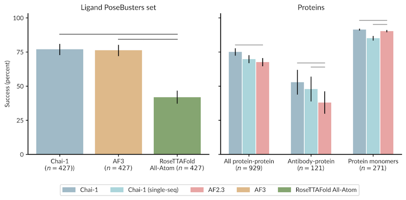
蛋白的序列文件,FASTA格式,支持多条序列。
注意:多蛋白复合物结构预测,其氨基酸序列输入格式如下:
>protein1
AASJ...
>protein2
AASJ...
>peptide
ASDF...
DNA核酸的序列文件,FASTA格式,支持多条序列。
RNA核酸分子的序列文件,FASTA格式,支持多条序列。
备注:当前24GB的GPU显存能计算的残基/碱基数量在1000个左右。
在Protein、DNA、RNA序列中,都支持残基或碱基的修饰,用CCD进行定义,CCD的介绍参考https://www.wwpdb.org/data/ccd 编号查询网址为https://www.ebi.ac.uk/pdbe-srv/pdbechem/
定义残基或碱基修饰时,直接在序列中用英文括号‘()’包含CCD code即可,示例如下:
>seq
(ACE)GQLEEIAK
表示在序列的N端发生了乙酰化;
>seq
AGSHSMRYFSTSVSR(HY3)GRGEPRFIAVG
表示序列中的残基P发生了羟基化修饰,变成HY3(CCD code)
文本文件包含小分子的结构信息,用SMILES格式,支持多个小分子,每行放置一个,示例如下:
CC(=O)OC1C[NH+]2CCC1CC2
[Mg+2]
注意:不适用于配体蛋白或多肽的氨基酸序列格式输入。
包含残基间距离限制信息的文本文件。距离限制的类型有两种:两个残基间的距离限制,一个残基与一条链之间的距离限制。
两个残基间的距离限制的定义由五部分组成:
五部分由逗号分隔,例如:1,R84,3,G7,10.0
表示第1条序列中的84号残基R,与第3条序列中的7号残基G,之间的最大距离为10.0埃。
一个残基与一条链之间的距离限制表示该残基与链中任意一个残基的距离满足限制即可。其定义方式与上述类似,差异在于,残基1与残基2的符号及位置编号,其中一个需设置为0(不可同时为0),例如:1,R84,3,0,10.0
表示第1条序列中的84号残基R,与第3条链的任意一个残基/碱基的最大距离为10.0埃即可。
支持放置多个距离限制,每行放置一个即可,包含多个距离限制信息的文件内容示例如下:
1,H189,3,L4,8.0
1,R84,3,0,10.0
是否使用MSA信息,默认使用。选择不使用时,则不会进行MSA查询,会使用ESM2特征代替MSA信息。
随机数种子,用于控制预测过程中的随机性。
输出结果文件为排名前5的复合物结构rank_1-5.cif和pred_scores_chai1.csv,csv中包含信息如下:
| 列名 | 说明 |
|---|---|
| Name | 结构名称 |
| Aggregate_Score | 对预测结构的质量排序的指标分数,值范围在-100至1.0之间,越大表示预测结构的质量越高。该分数综合考虑了三个指标:ptm, iptm, has_clash, 计算公式为: Aggregate_Score = 0.8 × ipTM + 0.2 × pTM − 100 × has_clash。注意:结构为单体时,因为ipTM为0,整体的综合得分偏低,可参考pTM即可。 |
| pTM | 预测的TM分数(the predicted template modeling score),衡量预测结构整体准确性,越大表示越准确,该分数大于0.5时,表示结构整体折叠可能与真实结构相似 |
| ipTM | 预测的亚基接触面的TM分数(the interface predicted template modeling score),当预测结构为复合物时才有该评价指标,衡量复合物中各个亚基之间相对位置的预测准确性,越大表示越准确,大于0.8表示高质量预测,小于0.6表示预测可能失败,0.6-0.8为灰色地带,预测正确与否不确定 |
| Avg_pAE | 平均pae分数,pae是预测对齐误差,是残基对水平的置信度指标,用来衡量任意两个残基之间相对空间位置的预测可信度。数值<5,表示残基对之间相对位置预测非常可靠,通常位于同一结构域内;数值在5–10,表示预测较为准确,可能为柔性环区或轻微构象差异区域;数值在10–20,表示相对位置不确定性较高,常见于结构域间连接区或柔性区域;数值> 20,表示预测不可靠,可能为无序区域、错误折叠,或复合物界面不稳定。 |
| Min_pAE | 所有pae分数中的最小值 |
| Avg_iPAE | 结构中相互作用界面的平均pae分数 |
| Min_iPAE | 结构中相互作用界面pae分数中的最小值 |
| pDockQ2_链名 | 该链的预测对接评分(pDock2),用于评估该链在复合物界面中的结合可靠性 |
| pDock2_Avg | 链之间的平均预测对接评分,用于整体评估复合物界面质量 |
| pDockQ2 范围 | 结构质量评估 |
|---|---|
| < 0.23 | 不正确(Incorrect) |
| 0.23 – 0.49 | 可接受(Acceptable) |
| 0.49 – 0.80 | 中等质量(Medium) |
| > 0.80 | 高质量(High quality) |
Based on Chai-1 structure prediction model implementation. Chai-1 is a multimodal basis model for molecular structure prediction that performs well on various benchmarks and can predict including proteins, small molecules, DNA, RNA, glycosylation, and more.
The sequence file of proteins in FASTA format, supporting multiple sequences.
Note: For multi-protein complex structure prediction, the amino acid sequence input format is as follows:
>protein1
AASJ...
>protein2
AASJ...
>peptide
ASDF...
The sequence file of DNA nucleic acids in FASTA format, supporting multiple sequences.
The sequence file of RNA nucleic acid molecules in FASTA format, supporting multiple sequences.
** Note: Current 24GB GPU memory can calculate around 1000 residues/bases. **
In Protein, DNA, RNA sequences, all support the modification of residues or bases, which are defined by CCD, The introduction of the CCD reference https://www.wwpdb.org/data/ccd Number query url for https://www.ebi.ac.uk/pdbe-srv/pdbechem/
To define a residue or base modification, simply include the CCD code in parentheses’ () 'in the sequence, as shown in the following example:
>seq
(ACE)GQLEEIAK
Indicates acetylation at the N-terminus of the sequence;
>seq
AGSHSMRYFSTSVSR(HY3)GRGEPRFIAVG
Indicates that residue P in the sequence is hydroxylated and becomes HY3 (CCD code).
The text file contains structural information about small molecules, in SMILES format, supporting multiple small molecules, one per line, as shown in the following example:
CC(=O)OC1C[NH+]2CCC1CC2
[Mg+2]
Note: Not applicable for amino acid sequence format input of ligand proteins or polypeptides.
The five parts are separated by commas, for example: 1,R84,3,G7,10.0
Denote residue 84 R in the first sequence, and residue 7 G in the third sequence, with a maximum distance of 10.0 angstroms.
** The distance limit between a residue and a chain ** means that the distance between the residue and any residue in the chain satisfies the limit. It is defined in the same way as above, except that the symbol and position number of residue 1 and residue 2 need to be set to 0 (not both), e.g. 1,R84,3,0,10.0
Denotes residue 84 R in the first sequence, and a maximum distance of 10.0 angstroms from any residue/base of the third strand is sufficient.
Multiple distance limits are supported, one per line, and an example file containing multiple distance limits is as follows:
1,H189,3,L4,8.0
1,R84,3,0,10.0
Whether to use MSA information; enabled by default.
If you choose not to use it, no MSA search will be performed and ESM2 features will be used instead of MSA information.
Random seed used to control the randomness in the prediction process.
The output files are the top 5 complex structures rank_1-5.cif and pred_scores_chai1.csv, which contain the following information:
| Field Name | Description |
|---|---|
| Name | Name of the complex structure |
| Aggregate_Score | Index scores that rank the quality of the predicted structure, with values ranging from -100 to 1.0, with larger values indicating higher quality of the predicted structure. The score takes into account three metrics: ptm, iptm, has_clash, and is calculated as follows: Aggregate_Score = 0.8 × ipTM + 0.2 × pTM − 100 × has_clash. Note: When the structure is monomeric, the Aggregate_Score is relatively low because ipTM is 0. In such cases, you can refer to pTM alone. |
| pTM | The predicted template modeling score, which measures the overall accuracy of the predicted structure. A higher score indicates greater accuracy. If the score is greater than 0.5, it suggests that the overall folding of the structure may be similar to the true structure. |
| ipTM | The interface predicted template modeling score, which measures the accuracy of the predicted relative positions of the subunits in the complex. A higher score indicates greater accuracy. Scores above 0.8 indicate high-quality predictions, while scores below 0.6 suggest potential failure of the prediction. Scores between 0.6 and 0.8 are in a gray area, where the accuracy of the prediction is uncertain. |
| Avg_pAE | Average pAE score; pAE stands for Predicted Aligned Error, a residue-pair-level confidence metric measuring the prediction reliability of relative spatial positions between any two residues. Values <5 indicate highly reliable predictions of relative positions between residue pairs, typically within the same domain; values of 5–10 suggest relatively accurate predictions, possibly in flexible loop regions or areas with minor conformational differences; values of 10–20 indicate high uncertainty in relative positions, commonly found in inter-domain linkers or flexible regions; values >20 indicate unreliable predictions, possibly representing disordered regions, misfolding, or unstable complex interfaces. |
| Min_pAE | The minimum value among all pAE scores. |
| Avg_iPAE | The average value of interface pAE scores. |
| Min_iPAE | The minimum value among all ipAE scores. |
| pDockQ2_chain | Predicted docking score (pDockQ2) for a specific chain, used to evaluate the reliability of that chain’s interaction at the complex interface |
| pDock2_Avg | Average predicted docking score between chains, used to assess the overall interface quality of the complex |
| pDockQ2 Range | Structure Quality Assessment |
|---|---|
| < 0.23 | Incorrect |
| 0.23 – 0.49 | Acceptable |
| 0.49 – 0.80 | Medium quality |
| > 0.80 | High quality |

ADMET Prediction (v2)是一个基于机器学习的小分子ADMET性质预测模块。能快速批量预测小分子的ADMET性质,支持图注意力神经网络模型(GNN)、轻量梯度提升树模型(LGBM)、随机森林模型(RF)、梯度提升树模型(XGBT)4种常见高效的机器学习算法,分子特征支持分子指纹(Morgan FP)以及分子描述符(Descriptors)两种方法,能对小分子化合物库进行快速批量预测。模块支持27种ADMET性质,其中7种回归模型,20种分类模型。不同机器学习方法以及分子特征化方法预测性能如下:
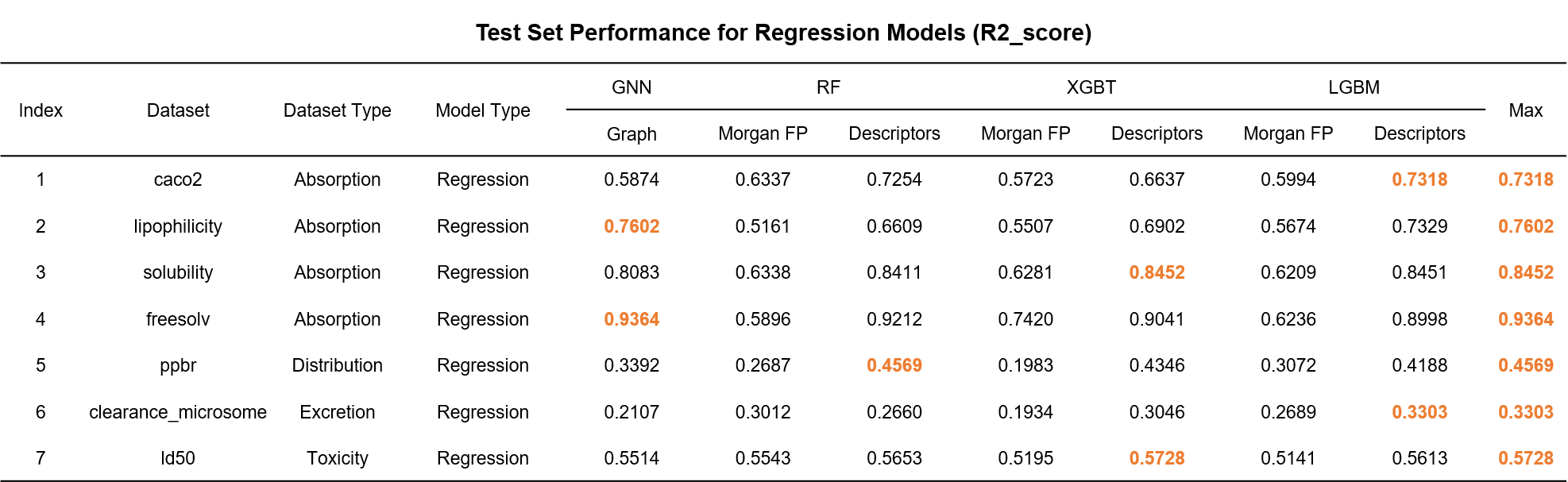
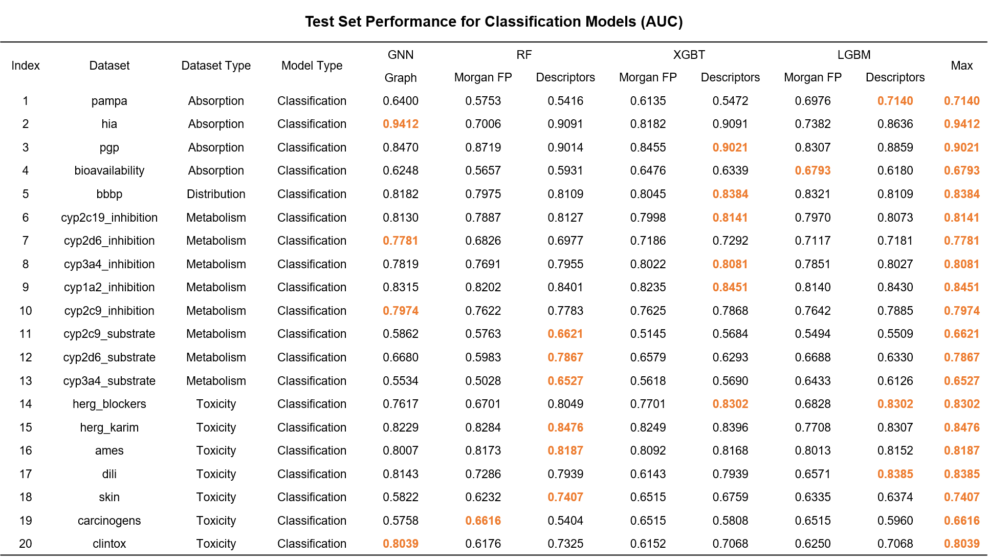
模块自动选择最理想的机器学习算法和分子特征化方法的组合进行预测。
待预测的小分子文件,SDF格式。
ADMET预测列表,ADMET性质见结果说明部分。
输出的预测结果文件,默认为predicted_results.csv
输出结果中,如果是分类模型,输出0或1分类。如果是回归模型,预测出实际值。
ADMET性质信息如下:
| Dataset | Dataset Abbr. | ADMET Type | Dataset Type | Endpoints Description |
|---|---|---|---|---|
| Caco-2 (Cell Effective Permeability), Wang et al. | caco2 | Absorption | Regression | logPapp |
| PAMPA Permeability, NCATS | pampa | Absorption | Binary classification | high permeability (1) or low-to-moderate permeability (0) in PAMPA assay |
| HIA (Human Intestinal Absorption), Hou et al. | hia | Absorption | Binary classification | good permeability (1) or poor permeability (0) |
| Pgp (P-glycoprotein) Inhibition, Broccatelli et al. | pgp | Absorption | Binary classification | inhibitor (1) or non-inhibitor (0) |
| Bioavailability, Ma et al. | bioavailability | Absorption | Binary classification | High (1) or low (0) bioavailability |
| Lipophilicity, AstraZeneca | lipophilicity | Absorption | Regression | octanol/water distribution coefficient (logD at pH 7.4) |
| Solubility, AqSolDB | solubility | Absorption | Regression | logS |
| Hydration Free Energy, FreeSolv | freesolv | Absorption | Regression | Hydration Free Energy (kcal/mol) |
| BBB (Blood-Brain Barrier), Martins et al. | bbbp | Distribution | Binary classification | High (1) or low (0) blood-brain barrier penetration |
| PPBR (Plasma Protein Binding Rate), AstraZeneca | ppbr | Distribution | Regression | Plasma Protein Binding Rate (0-100) |
| CYP P450 2C19 Inhibition, Veith et al. | cyp2c19_inhibition | Metabolism | Binary Classification | P450 2C19 inhibitor (1) or non-inhibitor (0) |
| CYP P450 2D6 Inhibition, Veith et al. | cyp2d6_inhibition | Metabolism | Binary Classification | P450 2D6 inhibitor (1) or non-inhibitor (0) |
| CYP P450 3A4 Inhibition, Veith et al. | cyp3a4_inhibition | Metabolism | Binary Classification | P450 3A4 inhibitor (1) or non-inhibitor (0) |
| CYP P450 1A2 Inhibition, Veith et al. | cyp1a2_inhibition | Metabolism | Binary Classification | P450 1A2 inhibitor (1) or non-inhibitor (0) |
| CYP P450 2C9 Inhibition, Veith et al. | cyp2c9_inhibition | Metabolism | Binary Classification | P450 2C9 inhibitor (1) or non-inhibitor (0) |
| CYP2C9 Substrate, Carbon-Mangels et al. | cyp2c9_substrate | Metabolism | Binary Classification | CYP2C9 substrate (1) or non-substrate (0) |
| CYP2D6 Substrate, Carbon-Mangels et al. | cyp2d6_substrate | Metabolism | Binary Classification | CYP2CD6 substrate (1) or non-substrate(0) |
| CYP3A4 Substrate, Carbon-Mangels et al. | cyp3a4_substrate | Metabolism | Binary Classification | CYP3A4 substrate (1) or non-substrate(0) |
| Microsome Clearance, AstraZeneca | clearance_microsome | Excretion | Regression | Microsome Clearance (CL) |
| Acute Toxicity LD50 | ld50 | Toxicity | Regression | Acute Toxicity LD50 |
| hERG blockers | herg_blockers | Toxicity | Binary classification | hERG blockers (1) or non-blockers (0) |
| hERG Karim et al. | herg_karim | Toxicity | Binary classification | hERG blockers (1) or non-blockers (0) |
| Ames Mutagenicity | ames | Toxicity | Binary classification | high (1) or low (0) ames mutagenicity |
| DILI (Drug Induced Liver Injury) | dili | Toxicity | Binary classification | high (1) or low (0) drug induced liver injury |
| Skin Reaction | skin | Toxicity | Binary classification | high (1) or low (0) skin reaction |
| ClinTox | clintox | Toxicity | Binary classification | high (1) or low (0) ClinTox |
| Carcinogens | carcinogens | Toxicity | Binary classification | high (1) or low (0) Carcinogens |
ADMET Prediction (v2) is a machine learning-based module for predicting the ADMET properties of small molecules. It enables rapid batch predictions of ADMET properties and supports four common and efficient machine learning algorithms: Graph Attention Neural Network (GAT), Light Gradient Boosting Machine (LightGBM), Random Forest, and Gradient Boosting Machine (GBM). The module supports two methods for molecular feature representation: molecular fingerprints and molecular descriptors, allowing for quick batch predictions on libraries of small molecule compounds. It supports 27 ADMET properties, including 7 regression models and 20 classification models. Users can select the ideal machine learning algorithm and molecular characterization method based on the predictive performance data provided in the documentation. The predictive performance of different machine learning methods and molecular characterization methods is as follows:
The module selects the ideal machine learning algorithm and molecular characterization method automaticaly based on the predictive performance data provided in the documentation.
Small molecular structure file in SDF format
ADMET properties. Details can be seen in results.
Output prediction results file name with default predicted_results.csv
In the output results, if it is a classification model, the output will be a classification of 0 or 1. The predicted output will be the actual value if it is a regression model. The endpoint descriptions are as follows:
| Dataset | Dataset Abbr. | ADMET Type | Dataset Type | Endpoints Description |
|---|---|---|---|---|
| Caco-2 (Cell Effective Permeability), Wang et al. | caco2 | Absorption | Regression | logPapp |
| PAMPA Permeability, NCATS | pampa | Absorption | Binary classification | high permeability (1) or low-to-moderate permeability (0) in PAMPA assay |
| HIA (Human Intestinal Absorption), Hou et al. | hia | Absorption | Binary classification | good permeability (1) or poor permeability (0) |
| Pgp (P-glycoprotein) Inhibition, Broccatelli et al. | pgp | Absorption | Binary classification | inhibitor (1) or non-inhibitor (0) |
| Bioavailability, Ma et al. | bioavailability | Absorption | Binary classification | High (1) or low (0) bioavailability |
| Lipophilicity, AstraZeneca | lipophilicity | Absorption | Regression | octanol/water distribution coefficient (logD at pH 7.4) |
| Solubility, AqSolDB | solubility | Absorption | Regression | logS |
| Hydration Free Energy, FreeSolv | freesolv | Absorption | Regression | Hydration Free Energy (kcal/mol) |
| BBB (Blood-Brain Barrier), Martins et al. | bbbp | Distribution | Binary classification | High (1) or low (0) blood-brain barrier penetration |
| PPBR (Plasma Protein Binding Rate), AstraZeneca | ppbr | Distribution | Regression | Plasma Protein Binding Rate (0-100) |
| CYP P450 2C19 Inhibition, Veith et al. | cyp2c19_inhibition | Metabolism | Binary Classification | P450 2C19 inhibitor (1) or non-inhibitor (0) |
| CYP P450 2D6 Inhibition, Veith et al. | cyp2d6_inhibition | Metabolism | Binary Classification | P450 2D6 inhibitor (1) or non-inhibitor (0) |
| CYP P450 3A4 Inhibition, Veith et al. | cyp3a4_inhibition | Metabolism | Binary Classification | P450 3A4 inhibitor (1) or non-inhibitor (0) |
| CYP P450 1A2 Inhibition, Veith et al. | cyp1a2_inhibition | Metabolism | Binary Classification | P450 1A2 inhibitor (1) or non-inhibitor (0) |
| CYP P450 2C9 Inhibition, Veith et al. | cyp2c9_inhibition | Metabolism | Binary Classification | P450 2C9 inhibitor (1) or non-inhibitor (0) |
| CYP2C9 Substrate, Carbon-Mangels et al. | cyp2c9_substrate | Metabolism | Binary Classification | CYP2C9 substrate (1) or non-substrate (0) |
| CYP2D6 Substrate, Carbon-Mangels et al. | cyp2d6_substrate | Metabolism | Binary Classification | CYP2CD6 substrate (1) or non-substrate(0) |
| CYP3A4 Substrate, Carbon-Mangels et al. | cyp3a4_substrate | Metabolism | Binary Classification | CYP3A4 substrate (1) or non-substrate(0) |
| Microsome Clearance, AstraZeneca | clearance_microsome | Excretion | Regression | Microsome Clearance (CL) |
| Acute Toxicity LD50 | ld50 | Toxicity | Regression | Acute Toxicity LD50 |
| hERG blockers | herg_blockers | Toxicity | Binary classification | hERG blockers (1) or non-blockers (0) |
| hERG Karim et al. | herg_karim | Toxicity | Binary classification | hERG blockers (1) or non-blockers (0) |
| Ames Mutagenicity | ames | Toxicity | Binary classification | high (1) or low (0) ames mutagenicity |
| DILI (Drug Induced Liver Injury) | dili | Toxicity | Binary classification | high (1) or low (0) drug induced liver injury |
| Skin Reaction | skin | Toxicity | Binary classification | high (1) or low (0) skin reaction |
| ClinTox | clintox | Toxicity | Binary classification | high (1) or low (0) ClinTox |
| Carcinogens | carcinogens | Toxicity | Binary classification | high (1) or low (0) Carcinogens |

Evaluate Nucleic Acid (AlphaRNA)模块用于评估核酸序列的其表达量和半衰期、抗体滴度等。支持人、小鼠、大鼠、猪等种属。
核酸序列,必须为3的倍数,否则截断尾部序列以达到3的倍数序列,比如:GGAGCCGAGGCGGGCCGATTCACGATCGGTTCGCAAAAACTGTTTGGG
序列所属物种,Homo_Sapiens、Mamalian、Pig、Rat。
输出结果文件为result.csv,包含信息如下:
| 字段名称 | 说明 |
|---|---|
| AUP | AUP (Amino Acid Usage Pattern)指的是氨基酸使用模式的指标,通常用于评估特定氨基酸在序列中的使用频率。值越高,表示该氨基酸在序列中使用的频率越高。 |
| CAI | CAI (Codon Adaptation Index)是一个用于评估特定基因的密码子使用偏好度的指标,值范围从 0 到 1。接近 1 表示该基因的密码子使用模式与高表达基因的模式相似,通常与基因表达效率相关。 |
| GCR | GCR (Gene Codon Ratio)是基因密码子比率的指标,反映了基因中不同密码子的相对使用情况。值越高,表示基因中使用的密码子与参考密码子库的偏好越一致。 |
| MFE | MFE (Minimum Free Energy)是指核酸序列的最低自由能,通常用于评估 RNA 二级结构的稳定性。值越低表示结构越稳定。负值表示该序列在折叠时释放能量,形成稳定的构象。 |
| Aug Positions | Aug Positions表示在序列中发现的AUG(起始密码子)的位置。结果空时表示在序列中没有找到AUG密码子。 |
| Sequence | 根据输入的核酸序列翻译得到的氨基酸序列。 |
| Secondary Structure | RNA序列的预测二级结构。 |
The Evaluate Nucleic Acid (AlphaRNA) module is used to assess the expression levels, half-lives, antibody titers, and other characteristics of nucleic acid sequences.
The nucleic acid sequence must be a multiple of three; otherwise, the tail of the sequence will be truncated to achieve a length that is a multiple of three. For example: GGAGCCGAGGCGGGCCGATTCACGATCGGTTCGCAAAAACTGTTTGGG.
The species to which the sequence belongs, such as Homo_Sapiens, Mammalian, Pig, or Rat.
The output result file is result.csv, which contains the following information:
| Field Name | Description |
|---|---|
| AUP | AUP (Amino Acid Usage Pattern) indicates the usage pattern of amino acids, typically used to assess the frequency of specific amino acids in the sequence. A higher value indicates a higher frequency of that amino acid in the sequence. |
| CAI | CAI (Codon Adaptation Index) is a metric used to evaluate the codon usage preference of a specific gene, with values ranging from 0 to 1. A value close to 1 indicates that the codon usage pattern of the gene is similar to that of highly expressed genes, which is often related to gene expression efficiency. |
| GCR | GCR (Gene Codon Ratio) is an indicator of the gene codon ratio, reflecting the relative usage of different codons within the gene. A higher value indicates that the codons used in the gene are more consistent with the preferences of the reference codon library. |
| MFE | MFE (Minimum Free Energy) refers to the minimum free energy of the nucleic acid sequence, typically used to assess the stability of RNA secondary structures. Lower values indicate more stable structures. Negative values indicate that the sequence releases energy when folded, forming a stable conformation. |
| Aug Positions | Aug Positions indicates the positions of AUG (start codon) found in the sequence. An empty result means that no AUG codons were found in the sequence. |
| Sequence | The amino acid sequence translated from the input nucleic acid sequence. |
| Secondary Structure | The predicted secondary structure of the RNA sequence. |
Back Mutation Grouping是抗体人源化设计流程中分组模块,根据Mutation Score模块输出的回复突变评分表对回复突变进行分组,并返回突变后的序列。
抗体CDR区嫁接后序列文件,FASTA格式,由Grafting模块生成
抗体序列文件,FASTA格式
人源化突变评分文件,CSV格式,由Mutation Score模块生成
指定输出的突变序列文件名称,FASTA格式
打分分组的截断值,逗号分割,例如:2,5,10表示将氨基酸突变评分大于10的为一组,5~10的氨基酸为一组,小于2的氨基酸分为一组。
指定输出的回复突变的文件
根据不同截断值得到突变分组结果文件mutate_policy.json。
Back Mutation Grouping is a grouping module in the humanization design process of antibodies, which groups back mutations based on the mutation score table output by the Mutation Score module and returns the mutated sequences.
Sequence file of the antibody CDR region after grafting, in FASTA format, generated by the Grafting module.
Sequence file of the antibody, in FASTA format.
Humanization mutation score file, in CSV format, generated by the Mutation Score module.
Specify the name of the output mutation sequence file, in FASTA format.
Cutoff values for scoring grouping, separated by commas. For example, 2,5,10 indicates grouping amino acid mutations with scores greater than 10 in one group, amino acids with scores between 5 and 10 in another group, and amino acids with scores less than 2 in a separate group.
Specify the file for the output of back mutations.
The mutation grouping results file, mutate_policy.json, is generated based on different cutoff values.
基于自定义的蛋白结构模板,采用colabfold进行蛋白结构预测。
蛋白的序列文件,FASTA格式
蛋白的模板结构,PDB格式
| 输出文件名称 | 说明 |
|---|---|
| rank_001.pdb | 预测得到的最佳复合物结构。 |
| pdbs.tar.gz | 预测得到的前5个最佳复合物结构的压缩包文件。 |
| scores.csv | 预测结构的评分文件 |
其中scores.csv包含如下信息:
| 字段名称 | 说明 |
|---|---|
| Name | 预测结构的文件名 |
| pLDDT | 局部结构的可信度指标,值范围是0-100,该值越大说明预测的结构越可靠。低于70被认为可靠性较低,低于50基本认为是可信度非常低,为无序预测 |
| pTM | 预测的TM分数(the predicted template modeling score),衡量预测结构整体准确性,越大表示越准确,该分数大于0.5时,表示结构整体折叠可能与真实结构相似 |
| ipTM | 预测的亚基接触面的TM分数(the interface predicted template modeling score),当预测结构为复合物时才有该评价指标,衡量复合物中各个亚基之间相对位置的预测准确性,越大表示越准确,大于0.8表示高质量预测,小于0.6表示预测可能失败,0.6-0.8为灰色地带,预测正确与否不确定 |
Protein structure prediction is performed using ColabFold based on a custom protein structure template.
The sequence file of the protein in FASTA format.
The template structure of the protein in PDB format.
| Output File Name | Description |
|---|---|
| rank_001.pdb | The predicted best complex structure. |
| pdbs.tar.gz | A compressed file containing the top 5 best complex structures. |
| scores.csv | The scoring file for the predicted structures. |
The scores.csv file contains the following information:
| Field Name | Description |
|---|---|
| Name | The file name of the predicted structure. |
| pLDDT | The confidence score for local structure, with a range of 0-100. A higher value indicates a more reliable prediction. Values below 70 are considered low reliability, below 50 are generally regarded as very low confidence, indicating disordered predictions. |
| pTM | The predicted template modeling score, which measures the overall accuracy of the predicted structure. A higher score indicates greater accuracy. If the score is greater than 0.5, it suggests that the overall folding of the structure may be similar to the true structure. |
| ipTM | The interface predicted template modeling score, which measures the accuracy of the predicted relative positions of the subunits in the complex. A higher score indicates greater accuracy. Scores above 0.8 indicate high-quality predictions, while scores below 0.6 suggest potential failure of the prediction. Scores between 0.6 and 0.8 are in a gray area, where the accuracy of the prediction is uncertain. |
细胞免疫系统是人体免疫的重要组成部分,它使用 T 细胞受体 (TCR) 识别由主要组织相容性复合体 (MHC) 蛋白呈递的肽形式的抗原蛋白。准确定义TCR的结构基础及其与肽-MHC的结合可以为正常和异常免疫提供重要见解,并有助于指导疫苗和免疫疗法的设计。鉴于实验确定的TCR-肽-MHC结构数量有限,而每个个体内的TCR以及抗原靶标数量巨大,因此需要准确的建模方法。该模块基于TCRmodel2实现,TCRmodel2在AlphaFold基础上对TCR-肽-MHC复合物建模做了优化,与原生AlphaFold和其他基于基准测试的TCR-肽-MHC复合物建模方法相比,其准确度相似或更高,可在30分钟内完成复合物结构预测。
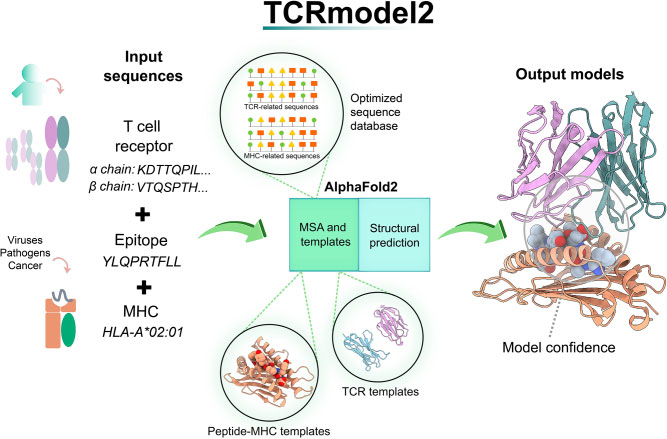
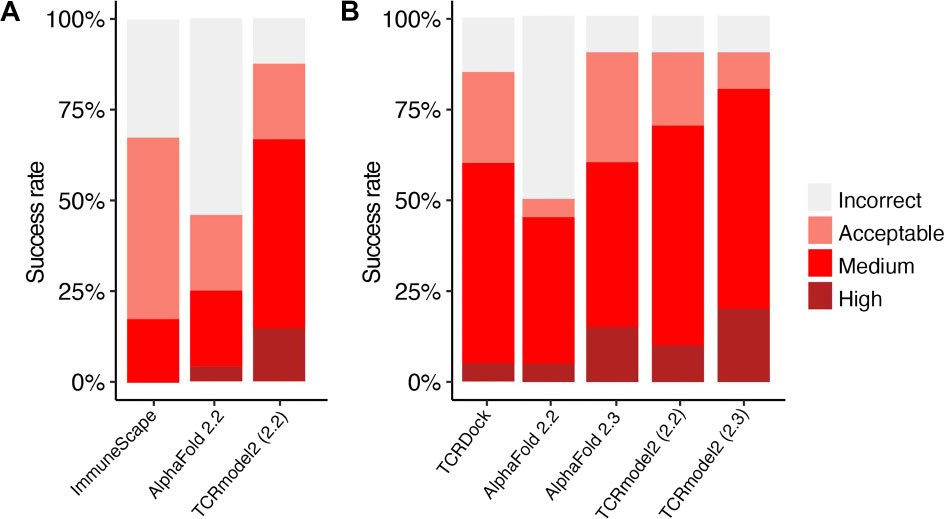
TCR α链的序列,如:AQEVTQIPAALSVPEGENLVLNCSFTDSAIYNLQWFRQDPGKGLTSLLLIQSSQREQTSGRLNASLDKSSGRSTLYIAASQPGDSATYLCAVTNQAGTALIFGKGTTLSVSS
TCR β链的序列,如:NAGVTQTPKFQVLKTGQSMTLQCSQDMNHEYMSWYRQDPGMGLRLIHYSVGAGITDQGEVPNGYNVSRSTTEDFPLRLLSAAPSQTSVYFCASSYSIRGSRGEQFFGPGTRLTVL
多肽序列,如:LAWEWWRTVAL
注:输入的多肽序列长度需要符合相应要求,如下:
I型TCR-pMHC复合物中,多肽的序列长度在8-15之间;
II型TCR-pMHC复合物中,多肽的长度为11。
MHC-I型序列或MHC-II α链序列。
当预测I型TCR-pMHC复合物时,输入MHC-I型序列,如:SHSLKYFHTSVSRPGRGEPRFISVGYVDDTQFVRFDNDAASPRMVPRAPWMEQEGSEYWDRETRSARDTAQIFRVNLRTLRGYYNQSEAGSHTLQWMHGCELGPDGRFLRGYEQFAYDGKDYLTLNEDLRSWTAVDTAAQISEQKSNDASEAEHQRAYLEDTCVEWLHKYLEKGKETLLH
当预测II型TCR-pMHC复合物时,输入MHC-II α链序列,如:IKADHVSTYAAFVQTHRPTGEFMFEFDEDEMFYVDLDKKETVWHLEEFGQAFSFEAQGGLANIAILNNNLNTLIQRSNHTQAT
MHC-II β链序列,当预测II型TCR-pMHC复合物时才需要输入,如:PENYLFQGRQECYAFNGTQRFLERYIYNREEFARFDSDVGEFRAVTELGRPAAEYWNSQKDILEEKRAVPDRMCRHNYELGGPMTLQR
输出结果包括:
| 输出文件名称 | 说明 |
|---|---|
| ranked_0.pdb | 预测得到的最佳复合物结构。 |
| pdbs.tar.gz | 预测得到的前5个最佳复合物结构的压缩包文件。 |
| scores.csv | 结构评分文件 |
其中scores.csv包含如下信息:
| 字段名称 | 说明 |
|---|---|
| PDB | 复合物PDB结构的文件名 |
| Model_Confidence | 结构的置信度评分,是pTM与ipTM评分的加权综合值,数值在0-1之间,越接近1表示结构模型质量越好 |
| pLDDT | 局部结构的可信度指标,值范围是0-100,该值越大说明预测的结构越可靠。低于70被认为可靠性较低,低于50基本认为是可信度非常低,为无序预测 |
| pTM | the predicted template modeling score预测的TM分数,衡量预测结构整体准确性,越大表示越准确,该分数大于0.5时,表示结构整体折叠可能与真实结构相似 |
| ipTM | the interface predicted template modeling score预测的亚基接触面的TM分数,衡量复合物中各个亚基之间相对位置的预测准确性,越大表示越准确,大于0.8表示高质量预测,小于0.6表示预测可能失败,0.6-0.8为灰色地带,预测正确与否不确定 |
| TCR-pMHC_ipTM | TCR与pMHC之间的ipTM值 |
The cellular immune system is a crucial component of the human immune response, utilizing T cell receptors (TCRs) to recognize peptide-form antigens presented by major histocompatibility complex (MHC) proteins. Accurately defining the structural basis of TCRs and their binding to peptide-MHC complexes can provide important insights into both normal and abnormal immune responses and assist in guiding the design of vaccines and immunotherapies. Given the limited number of experimentally determined TCR-peptide-MHC structures and the vast number of TCRs and antigen targets within each individual, accurate modeling methods are needed. This module is based on TCRmodel2, which optimizes TCR-peptide-MHC complex modeling on the foundation of AlphaFold. It achieves comparable or higher accuracy than native AlphaFold and other benchmark-based TCR-peptide-MHC modeling methods, completing complex structure predictions within 30 minutes.
The sequence of the TCR α chain, for example: AQEVTQIPAALSVPEGENLVLNCSFTDSAIYNLQWFRQDPGKGLTSLLLIQSSQREQTSGRLNASLDKSSGRSTLYIAASQPGDSATYLCAVTNQAGTALIFGKGTTLSVSS
The sequence of the TCR β chain, for example: NAGVTQTPKFQVLKTGQSMTLQCSQDMNHEYMSWYRQDPGMGLRLIHYSVGAGITDQGEVPNGYNVSRSTTEDFPLRLLSAAPSQTSVYFCASSYSIRGSRGEQFFGPGTRLTVL
The peptide sequence, for example: LAWEWWRTVAL.
Note: The length of the input peptide sequence must meet the following requirements:
For Class I TCR-pMHC complexes, the peptide sequence length should be between 8-15;
For Class II TCR-pMHC complexes, the peptide length is 11.
The MHC-I sequence or MHC-II α chain sequence.
When predicting Class I TCR-pMHC complexes, input the MHC-I sequence, for example: SHSLKYFHTSVSRPGRGEPRFISVGYVDDTQFVRFDNDAASPRMVPRAPWMEQEGSEYWDRETRSARDTAQIFRVNLRTLRGYYNQSEAGSHTLQWMHGCELGPDGRFLRGYEQFAYDGKDYLTLNEDLRSWTAVDTAAQISEQKSNDASEAEHQRAYLEDTCVEWLHKYLEKGKETLLH.
When predicting Class II TCR-pMHC complexes, input the MHC-II α chain sequence, for example: IKADHVSTYAAFVQTHRPTGEFMFEFDEDEMFYVDLDKKETVWHLEEFGQAFSFEAQGGLANIAILNNNLNTLIQRSNHTQAT.
The MHC-II β chain sequence, which is required only when predicting Class II TCR-pMHC complexes, for example: PENYLFQGRQECYAFNGTQRFLERYIYNREEFARFDSDVGEFRAVTELGRPAAEYWNSQKDILEEKRAVPDRMCRHNYELGGPMTLQR.
The output results include:
| Output File Name | Description |
|---|---|
| ranked_0.pdb | The predicted best complex structure. |
| pdbs.tar.gz | A compressed file containing the top 5 predicted complex structures. |
| scores.csv | Structure scoring file. |
The scores.csv contains the following information:
| Field Name | Description |
|---|---|
| PDB | The filename of the complex PDB structure. |
| Model_Confidence | The confidence score of the structure, which is a weighted composite value of pTM and ipTM scores, ranging from 0 to 1, with values closer to 1 indicating better model quality. |
| pLDDT | A measure of the reliability of the local structure, ranging from 0 to 100; higher values indicate more reliable predictions. Values below 70 are considered low reliability, and below 50 are deemed very low reliability, indicating disordered predictions. |
| pTM | The predicted template modeling score, which measures the overall accuracy of the predicted structure; higher values indicate greater accuracy. A score greater than 0.5 suggests that the overall folding of the structure may resemble the true structure. |
| ipTM | The interface predicted template modeling score, which measures the accuracy of the predicted relative positions of subunits within the complex; higher values indicate greater accuracy. Scores above 0.8 indicate high-quality predictions, while scores below 0.6 suggest potential failure, and scores between 0.6 and 0.8 are in a gray area where correctness is uncertain. |
| TCR-pMHC_ipTM | The ipTM value between the TCR and pMHC. |
Alanine Scan (MMPBSA)是计算丙氨酸突变后的结合自由能,并且提供能量分解数据、结合常数(Ka)、抑制剂常数(Ki)。熵的计算采用的是张增辉教授的相互作用熵的方法,该方法直接从分子动力学模拟计算结合自由能的熵组分(相互作用熵或-TΔS),但是需要选取结构稳定部分进行计算。
本模块提供四种计算方法,其中 Trajectory 是针对进行分子动力学模拟轨迹后计算其受配体之间的结合自由能;One Structure 是针对一帧pdb结构或者对接得到的PDB结构计算受配体之间的结合自由能,MMPBSA of One Structure 计算流程中可以直接输入PDB进行计算。
Index Name 是输入受配体组别名称;Custom Name 则是输入受配体的在PDB中的残基编号。
MD模拟后得到的路径文件,可以在GMX MD Run (GMX2023)模块或者AlphaAutoMD模块中获取。
受体名称,可以为Protein、DNA、RNA。
配体名称,可以为Protein、DNA、RNA。如果为小分子,填写其在PDB中的名称。如果体系中除了蛋白以外为配体(包括小分子)可用Other表示。
参考结构。默认system.gro。可以在GMX MD Run (GMX2024)模块的输出结果文件中找到。当周期性边界条件处理不当时可以使用该参数。
突变扫描为丙氨酸(ALA)的氨基酸位置。格式为‘32-34,36’。蛋白氨基酸或者核酸碱基序号从1开始重新编号,与初始pdb氨基酸编号无关。
丙氨酸扫描时使用的力场。
起始帧时间,单位ps。最好选取RMSD稳定时区进行计算,以消除结构不稳定时导致的整体熵偏大。
结束帧时间,单位ps。最好选取RMSD稳定时区进行计算,以消除结构不稳定时导致的整体熵偏大。
间隔时间,单位ps。
索引文件,ndx格式。当体系中存在膜结构的时候可以通过Membrane Solvation模块获取index.ndx文件。膜模拟中的受体为receptor,配体为ligand,膜为membrane。只能是AMBER力场下构建的膜体系才能进行计算。
定义受体组别进行结合能计算。组别中填写的为蛋白氨基酸或者核酸碱基的序号。例如1-213或者1-211,212-213。蛋白氨基酸或者核酸碱基序号从1开始重新编号,与初始pdb氨基酸编号无关。
定义配体组别进行结合能计算。组别中填写的为蛋白氨基酸或者核酸碱基的序号。例如1-213或者1-211,212-213。蛋白氨基酸或者核酸碱基序号从1开始重新编号,与初始pdb氨基酸编号无关。
拓扑文件,由MD Solvation模块或者Membrane Solvation模块得到。
结构文件,.gro格式,由MD Solvation模块或者Membrane Solvation模块得到。
体系参数压缩文件,tar.gz格式。由MD Solvation模块或者Membrane Solvation模块得到。
输出结果包括:
| 输出文件名称 | 说明 |
|---|---|
| MMPBSA_result.csv/MMPBSA_Result_txt.tar.gz | 丙氨酸突变结果csv文件。 |
| MMPBSA_Residue.csv/MMPBSA_Residue_csv.tar.gz | 残基能量分解数据(CSV)。 |
| MMPBSA.pdb/MMPBSA_pdb.tar.gz | 突变后能量映射到 PDB 文件,可用于可视化结合能贡献区域。 |
| MMPBSA.tar.gz | 全部原始数据,包括: • _mmpbsa_residue_#.txt(7 类能量:VDW、ELE、PB、SA、MM、PBSA、Binding)• _mmpbsa_residue.txt(残基能量汇总,对应 MMPBSA_Residue.csv)• _mmpbsa_atom#.pdb(原子能量映射 PDB,类似 MMPBSA.pdb)。 |
| ALA_Scan_Results.csv | 丙氨酸扫描所有残基突变结果。 |
ALA_Scan_Results.csv,包含信息如下:
| 字段名称 | 说明 |
|---|---|
| index | 残基编号。 |
| Residue | 原始残基名称。 |
| Mutation Residue | 突变后的残基(通常为丙氨酸 ALA)。 |
| dH (kJ/mol) | 焓贡献。 |
| Tds (kJ/mol) | 熵贡献(TΔS)。 |
| dG (kJ/mol) | 结合自由能变化。决定结合强弱的关键指标。越负说明亲和力越强。 |
| Ki (µM/L) | 解离常数,结合亲和力的倒数。 |
| Ka (L/µM) | 结合常数,亲和力大小。 |
Ka 越大表示结合力强,Ki 越小表示抑制效果强。
GROMACS: High performance molecular simulations through multi-level parallelism from laptops to supercomputers. M. J. Abraham, T. Murtola, R. Schulz, S. Páll, J. C. Smith, B. Hess, E. Lindahl, SoftwareX, 1, (2015), 19-25.
Duan L, Liu X, Zhang JZ. Interaction Entropy: A New Paradigm for Highly Efficient and Reliable Computation of Protein-Ligand Binding Free Energy. J Am Chem Soc. 2016 May 4;138(17):5722-8.
https://github.com/Electrostatics/apbs/blob/main/docs/index.rst
Alanine Scan (MMPBSA) calculates the binding free energy after alanine mutations and provides energy decomposition data, binding constants (Ka), and inhibitor constants (Ki). The entropy calculation uses the method of interaction entropy proposed by Professor Zhang Zenghui, which directly calculates the entropy component of the binding free energy (interaction entropy or -TΔS) from molecular dynamics simulations, but requires selecting stable structural regions for calculation. This module provides four calculation methods. Among them, Trajectory calculates the binding free energy between the receptor and ligand after molecular dynamics simulation trajectories; One Structure calculates the binding free energy between the receptor and ligand for a single frame PDB structure or a docked PDB structure; MMPBSA of One Structure allows direct input of a PDB for calculation. Index Name is the input receptor-ligand group name, while Custom Name is the input residue numbers of the receptor-ligand in the PDB.
Path file obtained after MD simulation, available in the GMX MD Run (GMX2023) module or AlphaAutoMD module.
Name of the receptor, can be Protein, DNA, or RNA.
Name of the ligand, can be Protein, DNA, or RNA. If it is a small molecule, enter its name in the PDB. Use ‘Other’ if the system contains a ligand (including small molecules) other than proteins.
Reference structure. Default: system.gro.
This file can be found in the output results of the GMX MD Run (GMX2024) module.
Use this parameter when periodic boundary conditions are not handled properly.
The mutation scans for the amino acid location of alanine (ALA). Must followed the format is ‘32-34,36’. The protein amino acid or nucleic acid number is re-numbered from 1, independent of the initial pdb amino acid number.
Force field used for alanine scanning.
Start frame time in ps. It is best to select a stable RMSD region for calculation to eliminate large overall entropy caused by structural instability.
End frame time in ps. It is best to select a stable RMSD region for calculation to eliminate large overall entropy caused by structural instability.
Time interval in ps.
Index file in ndx format. When there is a membrane structure in the system, you can obtain the index.ndx file through the Membrane Solvation module. In membrane simulations, the receptor is ‘receptor’, the ligand is ‘ligand’, and the membrane is ‘membrane’. Only membrane systems built under the AMBER force field can be calculated.
Define receptor groups for binding energy calculation. Enter the sequence numbers of protein amino acids or nucleic acid bases in the group. For example, 1-213 or 1-211,212-213. Protein amino acid or nucleic acid base numbers start from 1 and are independent of the initial pdb amino acid numbering.
Define ligand groups for binding energy calculation. Enter the sequence numbers of protein amino acids or nucleic acid bases in the group. For example, 1-213 or 1-211,212-213. Protein amino acid or nucleic acid base numbers start from 1 and are independent of the initial pdb amino acid numbering.
Topology file obtained from the MD Solvation module or Membrane Solvation module.
Structure file in .gro format obtained from the MD Solvation module or Membrane Solvation module.
System parameter compression file in tar.gz format. Obtained from the MD Solvation module or Membrane Solvation module.
The output includes:
| File Name | Description |
|---|---|
| MMPBSA_result.csv / MMPBSA_Result_txt.tar.gz | Alanine mutation result (csv file). |
| MMPBSA_Residue.csv / MMPBSA_Residue_csv.tar.gz | Residue energy decomposition data (CSV). |
| MMPBSA.pdb / MMPBSA_pdb.tar.gz | Energy mapped onto the PDB file after mutation, useful for visualizing binding energy contribution regions. |
| MMPBSA.tar.gz | Complete raw data, including: • _mmpbsa_residue_#.txt (7 energy terms: VDW, ELE, PB, SA, MM, PBSA, Binding) • _mmpbsa_residue.txt (residue energy summary, corresponding to MMPBSA_Residue.csv) • _mmpbsa_atom#.pdb (atomic energy mapped PDB files, similar to MMPBSA.pdb). |
| ALA_Scan_Results.csv | Results of alanine scanning mutations for all residues. |
| Field Name | Description |
|---|---|
| index | Residue index number. |
| Residue | Original residue name. |
| Mutation Residue | Mutated residue (typically alanine, ALA). |
| dH (kJ/mol) | Enthalpy change. |
| Tds (kJ/mol) | Entropy term (TΔS). |
| dG (kJ/mol) | Binding free energy change, the key indicator of binding strength. The more negative the value, the stronger the affinity. |
| Ki (µM/L) | Dissociation constant, reciprocal of binding affinity. |
| Ka (L/µM) | Association constant, magnitude of binding affinity. |
Larger Ka indicates stronger binding affinity, while smaller Ki indicates stronger inhibitory effect.
GROMACS: High performance molecular simulations through multi-level parallelism from laptops to supercomputers. M. J. Abraham, T. Murtola, R. Schulz, S. Páll, J. C. Smith, B. Hess, E. Lindahl, SoftwareX, 1, (2015), 19-25.
Duan L, Liu X, Zhang JZ. Interaction Entropy: A New Paradigm for Highly Efficient and Reliable Computation of Protein-Ligand Binding Free Energy. J Am Chem Soc. 2016 May 4;138(17):5722-8.
https://github.com/Electrostatics/apbs/blob/main/docs/index.rst
Back Mutation Grouping是抗体人源化设计流程中分组模块,根据Mutation Score模块输出的回复突变评分表对回复突变进行分组,并返回突变后的序列。
抗体CDR区嫁接后序列文件,FASTA格式,由Grafting模块生成
抗体序列文件,FASTA格式
人源化突变评分文件,CSV格式,由Mutation Score模块生成
指定输出的突变序列文件名称,FASTA格式
打分分组的截断值,逗号分割,例如:2,5,10表示将氨基酸突变评分大于10的为一组,5~10的氨基酸为一组,小于2的氨基酸分为一组。
指定输出的回复突变的文件
根据不同截断值得到突变分组结果文件mutate_policy.json。
Back Mutation Grouping is a grouping module in the humanization design process of antibodies, which groups back mutations based on the mutation score table output by the Mutation Score module and returns the mutated sequences.
Sequence file of the antibody CDR region after grafting, in FASTA format, generated by the Grafting module.
Sequence file of the antibody, in FASTA format.
Humanization mutation score file, in CSV format, generated by the Mutation Score module.
Specify the name of the output mutation sequence file, in FASTA format.
Cutoff values for scoring grouping, separated by commas. For example, 2,5,10 indicates grouping amino acid mutations with scores greater than 10 in one group, amino acids with scores between 5 and 10 in another group, and amino acids with scores less than 2 in a separate group.
Specify the file for the output of back mutations.
The mutation grouping results file, mutate_policy.json, is generated based on different cutoff values.
.png)
Antibody Numbering v2是抗体编号模块,用于注释抗体可变区(Fv)或恒定区(包括 Fc), 支持几乎所有主流的抗体编号规则,如可变区广泛使用的Kabat、Chothia 和 IMGT,以及恒定区主要使用的EU规则。
该模式针对抗体的Fv区序列(包括重链 VH 和轻链 VL),通过指定编号规则(如 Kabat、Chothia、或 IMGT)对氨基酸残基进行标准化编号。
抗体序列文件,FASTA格式,支持多序列模式。
可变区编号规则,支持Kabat、Chothia、IMGT,可多选。
通常用于抗体恒定区的EU、Kabat标准化编号。
抗体序列文件,FASTA格式,支持多序列模式。
恒定区编号规则:eu,kabat。默认为eu。
| 输出文件名称 | 说明 |
|---|---|
output_chothia(imgt\kabat\martin).csv |
抗体可变区四种编号规则的csv文件 |
output_chothia(imgt\kabat\martin).json |
抗体可变区四种编号规则的json文件 |
output_nonfv.fasta |
当输入文件是完整抗体序列(包含Fv和Fc)时,自动识别出Fv区;并非Fv部分提取出来单独保存为output_nonfv.fasta。如果输入只包含Fv区,则不输出。 |
三种不同编号规则的csv文件,包含信息如下:
| 字段名称 | 说明 |
|---|---|
| molecule | 抗体序列名称 |
| chain_type | 抗体链类型:重链(VH)或者轻链(VL) |
| is_cdr | 判断是否为CDR区 |
| loc | 序列位置 |
| numbering | 序列编号 |
| insertion | 插入序列编号 |
| region | 抗体可变区类型:CDR1、CDR2或者CDR3 |
| domain | 区域 |
| 输出文件名称 | 说明 |
|---|---|
output_EU.csv |
抗体恒定区EU编号规则的csv文件 |
output_EU.json |
抗体恒定区EU编号规则的json文件 |
output_MatchRate.csv |
跟不同IgG亚型相似度 |
其中output_EU.csv文件,包含信息如下:
| 字段名称 | 说明 |
|---|---|
| Chain | 抗体序列链类型 |
| Position | 序列位置 |
| Eu numbering | 序列EU编号 |
| Residue | 抗体氨基酸缩写 |
| IgG1 Ref | IgG1氨基酸缩号 |
| Region | 抗体恒定类型:CH1、CH2、CH3、Hinge |
| Mutation(IgG1) | 原序列突变成IgG1的突变信息 |
注意:在 output_MatchRate.csv 文件中,如果 MatchRate_Global 数值偏低,说明该序列与标准 Fc 区域的相似性较差,可能并不是典型的 Fc 结构,而是linker 或随机插入的非 Fc 序列。
| 输出文件名称 | 说明 |
|---|---|
failed_to_number.fasta |
不能进行恒定区编号的fasta文件 |
output_fc_kabat.csv |
抗体恒定区Kabat编号规则的csv文件 |
output_fc_kabat.json |
抗体恒定区Kabat编号规则的json文件 |
其中output_fc_kabat.csv文件,包含信息如下:
| 字段名称 | 说明 |
|---|---|
| molecule | 抗体序列名称 |
| Residue | 抗体氨基酸缩写 |
| chain_type | 抗体链类型:重链(VH)或者轻链(VL) |
| is_cdr | 判断是否为CDR区 |
| loc | 序列位置 |
| numbering | 序列编号 |
| insertion | 插入序列编号 |
| region | 抗体可变区类型:CDR1、CDR2或者CDR3 |
| domain | 区域 |
Antibody Numbering v2 is the antibody numbering module for the annotations of antibody variable region (Fv) or constant region (including Fc). It supports almost all mainstream antibody numbering rules, such as Kabat, Chothia and IMGT, which are widely used in the variable region, and EU rules, which are mainly used in the constant region.
This mode is for the Fv region of antibodies (including heavy chain VH and light chain VL). Amino acid residues are standardized according to the specified numbering scheme (e.g., Kabat, Chothia, or IMGT).
Antibody sequence file in FASTA format. Multiple sequences are supported.
Variable region numbering schemes. Supports Kabat, Chothia, and IMGT. Multiple selections are allowed.
Typically used for EU or Kabat standardized numbering of antibody constant regions.
Antibody sequence file in FASTA format. Multiple sequences are supported.
Numbering scheme for constant regions: EU or Kabat. The default is EU.
| Output File Name | Description |
|---|---|
output_chothia(imgt\kabat\martin).csv |
CSV files for the four numbering schemes of antibody variable regions |
output_chothia(imgt\kabat\martin).json |
JSON files for the four numbering schemes of antibody variable regions |
output_nonfv.fasta |
When the input sequence contains a full antibody (Fv + Fc), the Fv region is automatically identified and the non-Fv region is saved to output_nonfv.fasta. If the input contains only the Fv region, this file is not generated. |
The CSV files for the three numbering schemes contain the following fields:
| Field Name | Description |
|---|---|
| molecule | Antibody sequence name |
| chain_type | Antibody chain type: heavy chain (VH) or light chain (VL) |
| is_cdr | Indicates whether the position belongs to a CDR |
| loc | Sequence position |
| numbering | Numbering index |
| insertion | Insertion code |
| region | Antibody variable region type: CDR1, CDR2, or CDR3 |
| domain | Region/domain |
| Output File Name | Description |
|---|---|
output_EU.csv |
CSV file following EU numbering rules for antibody constant regions |
output_EU.json |
JSON file following EU numbering rules for antibody constant regions |
| Match Rate | Similarity to different IgG subtypes |
The output_EU.csv file contains the following fields:
| Field Name | Description |
|---|---|
| Chain | Antibody chain type |
| Position | Sequence position |
| Eu numbering | EU numbering index |
| Residue | Amino acid residue |
| IgG1 Ref | IgG1 reference residue |
| Region | Antibody constant region type: CH1, CH2, CH3, or Hinge |
| Mutation(IgG1) | Mutation information compared to IgG1 |
Note:In the output_MatchRate.csv file, a low MatchRate_Global indicates that the sequence has poor similarity to canonical Fc regions. Such residues are likely not true Fc sequences, but instead may be linkers or randomly inserted non-Fc segments.
| Output File Name | Description |
|---|---|
failed_to_number.fasta |
FASTA sequences that could not be numbered |
output_fc_kabat.csv |
CSV file following Kabat numbering rules for antibody constant regions |
output_fc_kabat.json |
JSON file following Kabat numbering rules for antibody constant regions |
The output_fc_kabat.csv file contains the following fields:
| Field Name | Description |
|---|---|
| molecule | Antibody sequence name |
| Residue | Amino acid residue |
| chain_type | Antibody chain type: heavy chain (VH) or light chain (VL) |
| is_cdr | Indicates whether the position belongs to a CDR |
| loc | Sequence position |
| numbering | Numbering index |
| insertion | Insertion code |
| region | Antibody variable region type: CDR1, CDR2, or CDR3 |
| domain | Region/domain |
WeADApt (Wecomput ADA prediction) 是一种基于多模融合架构的免疫原性预测系统。该方法有机地将多个与免疫原性相关的模型融合,构成一个高效的免疫反应模拟系统,可准确地模拟蛋白、抗体、多肽、疫苗等生物药的免疫原性,并能鉴别潜在的免疫原性的T细胞表位(引起临床人体免疫应答的肽段)。
注:该模块非最新版本,通常推荐使用更新版本。
使用100多个临床及上市抗体的ADA数据的测试结果显示,预测的打分(MolScore)与ADA发生率的相关性达到R=0.68(下图)。
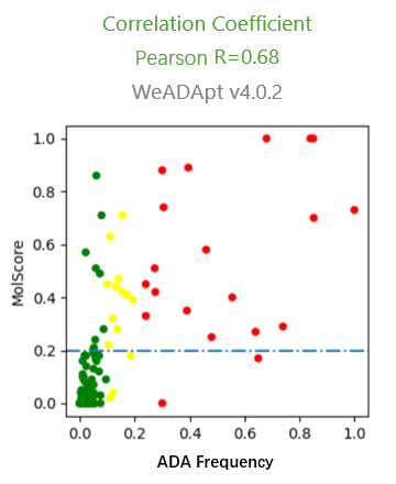
在同样的42个分子的数据集上,WeADApt预测的相关性超过了知名的商业软件EpiMatrix(R2=0.49 vs R2=0.42)。
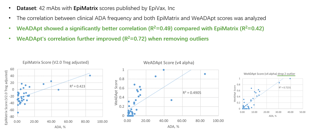
0.2分适合作为单抗的高/低风险的阈值(>20% ADA定义为高风险)。
这类分子仅需输入不重复的链即可
在唯信收集的双抗ADA数据集的测试表现如下图所示。以0.6的分数作为分界线,可以较好的区分高、低风险的双抗分子。双抗
注意,由于存在较多的B细胞清除双抗,其MOA会对ADA产生有较大的影响。
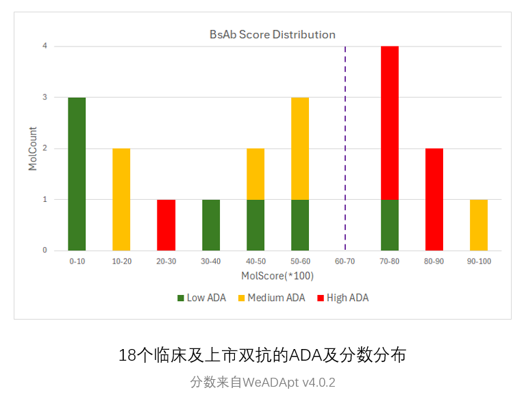
推荐从WeSeq中运行该功能,可以进行更多可视化交互

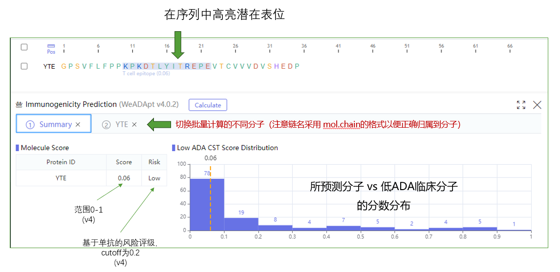
Score为预测的免疫原性风险评分(范围0-1),Risk为风险评级
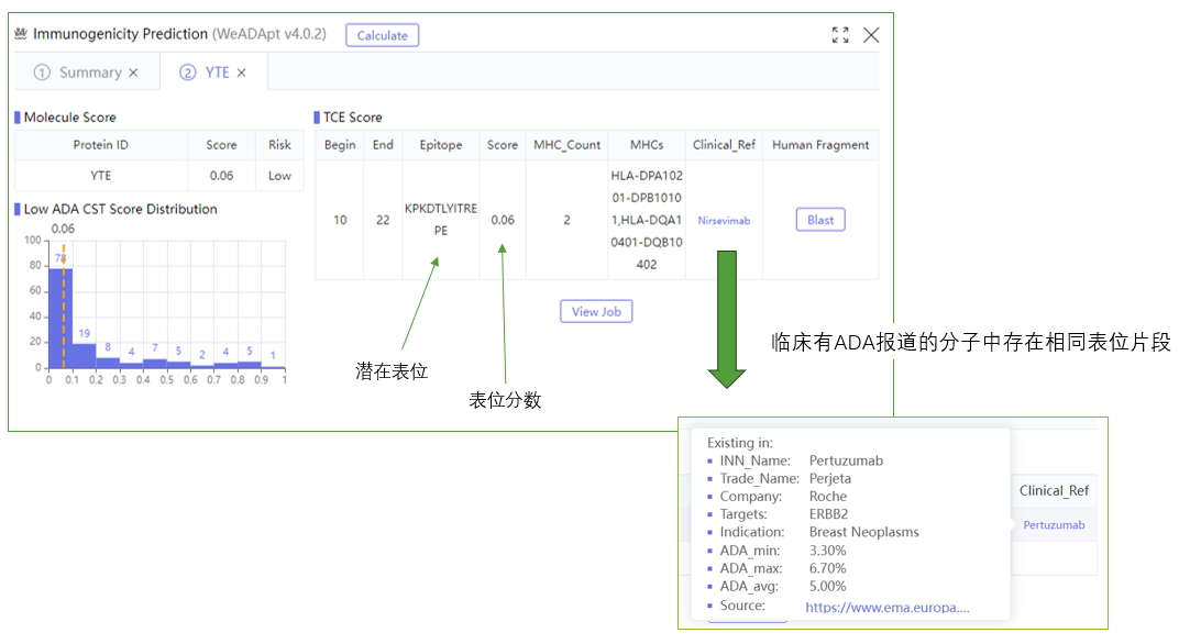
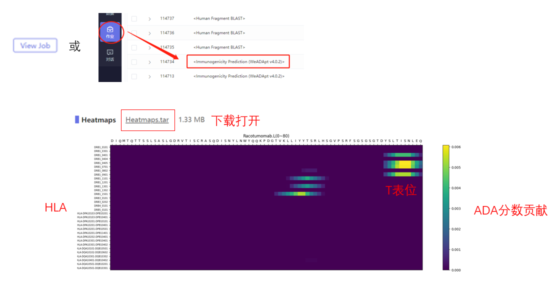
注意对照结构,排除不可及(包埋的)表位(下图)
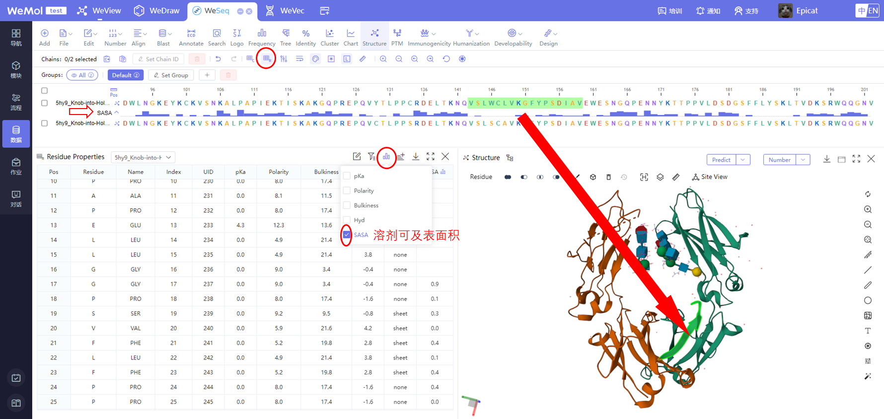
最简单的方式是进行人源片段的替换,可以直接在WeSeq中进行(下图)。
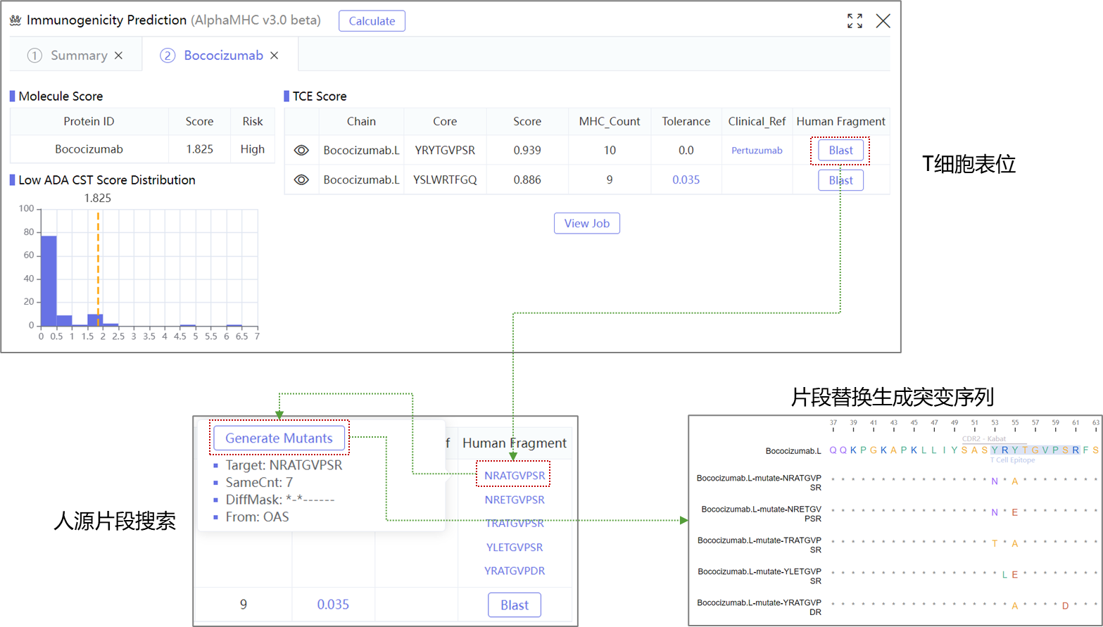
也可以通过频率分析功能引入人源突变。
突变完之后再对突变体预测一下免疫原性是否降低。
注意:从weseq中计算v4免疫原性的结果可以自动保存并且随时再打开的

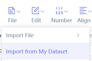
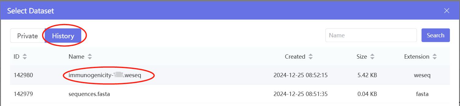
WeADApt (Wecomput ADA prediction) is an immunogenicity prediction system based on a multi-modal fusion architecture. This method organically integrates multiple models related to immunogenicity to form an efficient immune response simulation system. It can accurately simulate the immunogenicity of biologics such as proteins, antibodies, peptides, and vaccines, and identify potential immunogenic T-cell epitopes (peptide segments that elicit clinical human immune responses). PS: This module is not the latest version.
Testing results using ADA data from over 100 clinical and marketed antibodies show that the predicted scores (MolScore) correlate with ADA incidence at R=0.68 (see the figure below).
On the same dataset of 42 molecules, the correlation predicted by WeADApt exceeds that of the well-known commercial software EpiMatrix (R²=0.49 vs R²=0.42).
A score of 0.2 is suitable as a threshold for high/low risk in monoclonal antibodies (>20% ADA defined as high risk).
For these types of molecules, only non-redundant chains need to be input. The test performance on the bispecific ADA dataset collected by Weixin is shown in the figure below. With a score of 0.6 as the dividing line, high-risk and low-risk bispecific molecules can be better distinguished. Note that due to the presence of many B-cell depleting bispecifics, their MOA can significantly affect ADA.
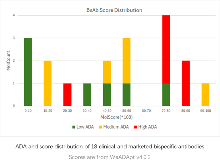
It is recommended to run this function from WeSeq for more visual interactions.
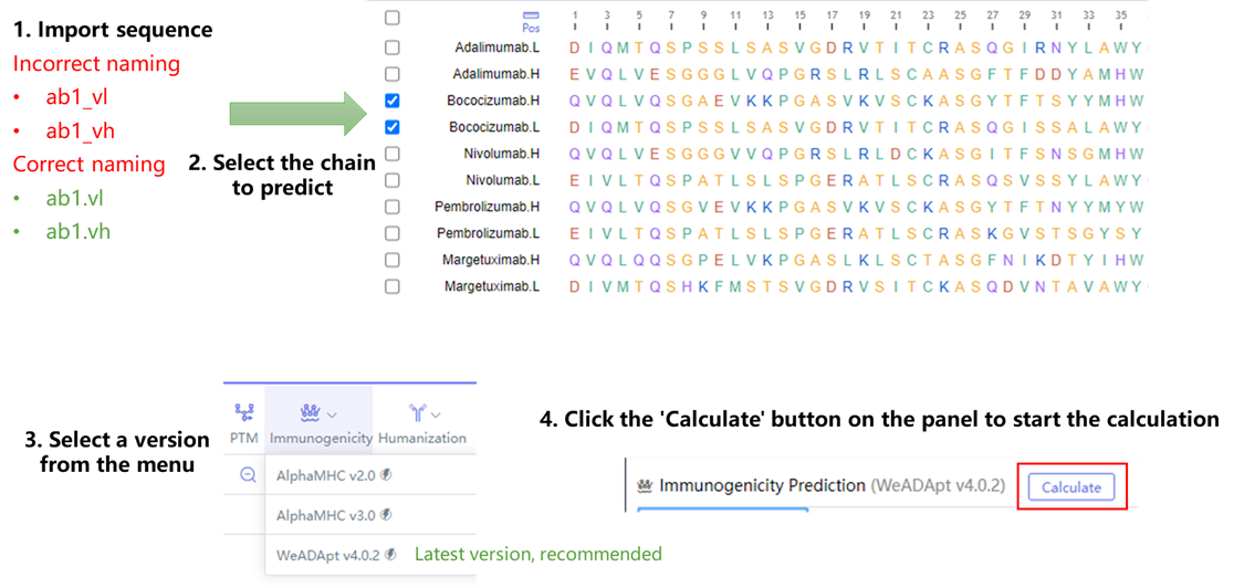

Score is the predicted immunogenicity risk score (range 0-1), and Risk is the risk rating.
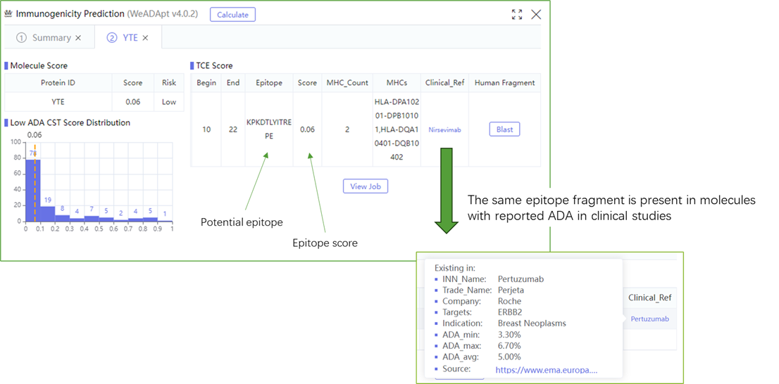
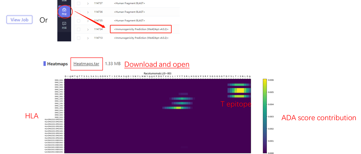
Note the reference structure and exclude inaccessible (embedded) epitopes (see the figure below).

The simplest way is to perform human fragment replacement, which can be done directly in WeSeq (see the figure below).
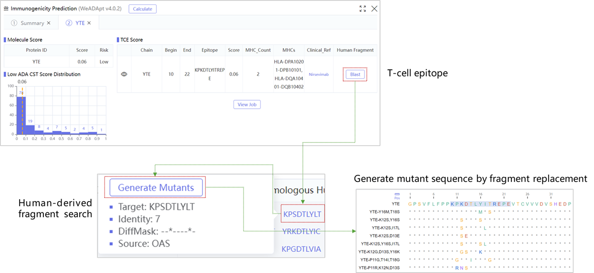
Human mutations can also be introduced through the frequency analysis feature. After mutation, predict the immunogenicity of the mutants to see if it has decreased.
Note: The results of calculating v4 immunogenicity in WeSeq can be automatically saved and reopened at any time.
Disulfide Bond Search模块计算蛋白质中潜在的二硫键位置,这对优化蛋白质的稳定性有所作用。二硫键作为对蛋白质的稳定性有极大的作用,但是加入不合理的二硫键也会容易引起聚集,表达量降低甚至错误折叠等不利影响。
在使用 PDB 格式的蛋白质结构文件时,如果其中存在缺失残基,请务必先通过Structure Preparation模块进行补全。若缺失未补全,直接输入可能导致报错。
指定需要设计的链,多条链用逗号分割,例如:A,B。
设置氨基酸序号,当参数Chain设置为A,C时,此参数如果设置为1 2 3 4 5 6 7 8 23 25, 10 11 12 13 14 15 16 17 18 19 20 40意味着对A中的残基1 2 3…25和链C中的残基10 11 12…40进行设计。如果不填,则该链的所有残基都参与设计。
注意:这里的氨基酸序号是从1开始,而不是PDB文件中带有的氨基酸序号。同一条链的氨基酸序号用空格分隔,不同链的氨基酸用逗号分隔。
是否只选择链间的二硫键。
可设置Cβ之间的距离,默认5.0Å。
输出结果包括:
| 输出文件名称 | 说明 |
|---|---|
| ss_bond.csv | 输出自然顺序编号、PDB文件中的残基编号以及Cβ之间的距离信息的CSV文件。 |
| ss_index.fasta | 序列名编号为自然顺序编号并将预测位点突变为CYS的FASTA文件。 |
| ss_uid.fasta | 序列名编号为PDB文件中的残基编号并将预测位点突变为CYS的的FASTA文件。 |
The Disulfide Bond Search module calculates potential disulfide bond positions in proteins, which can be useful for optimizing protein stability. Disulfide bonds play a significant role in stabilizing proteins, but improper addition of disulfide bonds can lead to aggregation, reduced expression levels, or even misfolding.
When using a protein structure file in PDB format, any missing residues must be completed in the Structure Preparation module before input. Failure to do so may result in errors.
Specify the chains to be designed. Multiple chains are separated by commas, e.g. A,B.
Set the amino acid sequence numbers. When the Chain parameter is set to A,C, setting this parameter to 1 2 3 4 5 6 7 8 23 25, 10 11 12 13 14 15 16 17 18 19 20 40 means designing residues 1 2 3...25 in chain A and residues 10 11 12...40 in chain C. If not specified, all residues in the chain will be included in the design.
Note: The amino acid sequence numbers here start from 1, not the residue numbers in the PDB file. Amino acid sequence numbers within the same chain are separated by spaces, and different chains are separated by commas.
Whether to select only interchain disulfide bonds.
The distance between Cβ atoms can be set, with a default of 5.0 Å.
The output includes:
| Output File Name | Description |
|---|---|
| ss_bond.csv | A CSV file containing information on the natural sequence number, residue number in the PDB file, and the distance between Cβ atoms. |
| ss_index.fasta | A FASTA file with sequence names numbered by natural sequence number, and predicted sites mutated to CYS. |
| ss_uid.fasta | A FASTA file with sequence names numbered by residue number in the PDB file, and predicted sites mutated to CYS. |

Pocket Finder模块基于几何特性和物理化学特性来识别这些口袋,其主要功能是快速、准确地识别蛋白质表面的潜在口袋。蛋白质口袋(或活性位点)是蛋白质表面的小区域,通常是药物分子或其他小分子结合的地方。识别这些口袋对于药物设计和蛋白质功能研究至关重要。
蛋白的结构文件,PDB格式。
最小alpha球的半径。
最大alpha球的半径。
距离阈值聚类算法
用于将Voronoi顶点分组的聚类方法:
s是单链接聚类(single linkage clustering)。m是完全链接聚类(complete linkage clustering)。a是平均链接聚类(average linkage clustering)。c是质心链接聚类(centroid linkage clustering)。聚类的距离度量方法:
e是欧几里得距离(euclidean distance)。b是曼哈顿距离(Manhattan distance)。每个口袋的最小alpha球数量。
输出结果包括:
| 输出文件名称 | 说明 |
|---|---|
| pocket_properties.csv | 口袋信息CSV文件 |
| pockets.tar.gz | 蛋白分析后得到的PDB文件压缩包 |
| pocket*_atm.pdb | 分别输出所有口袋的PDB(原子)文件格式 |
其中pocket_properties.csv包含如下信息:
| 字段名称 | 说明 |
|---|---|
| 口袋顺序 | |
| Score | 口袋综合得分,考虑了口袋的大小、形状和疏水性等因素。打分越高说明口袋更好,更有可能在生物学上具有相关性或适合药物结合。 |
| Druggability Score | 评估口袋结合药物分子的潜力,打分越高说明口袋药物可及性越高。 |
| Total SASA | 口袋可被溶剂分子接触的总表面积,单位为平方埃Ų;SASA较大,可容纳配体结构越大。 |
| Polar SASA | 总SASA中的极性部分,表示可被水分子接触的表面积。反映了口袋的亲水性。 |
| Apolar SASA | 总SASA中的非极性部分,表示不可被水分子接触的表面积。反映了口袋的疏水性。 |
| Volume | 口袋的体积,单位为ų。较大的体积表示口袋较大,能够容纳更大的配体或多个结合位点。 |
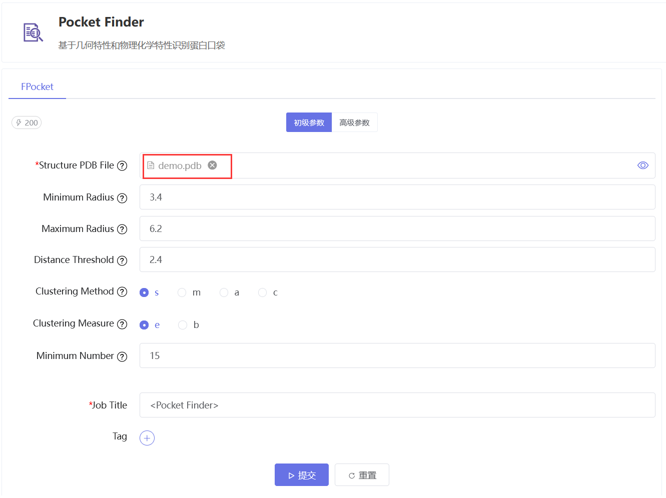
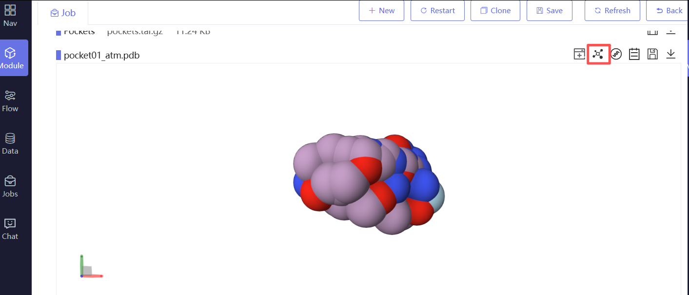
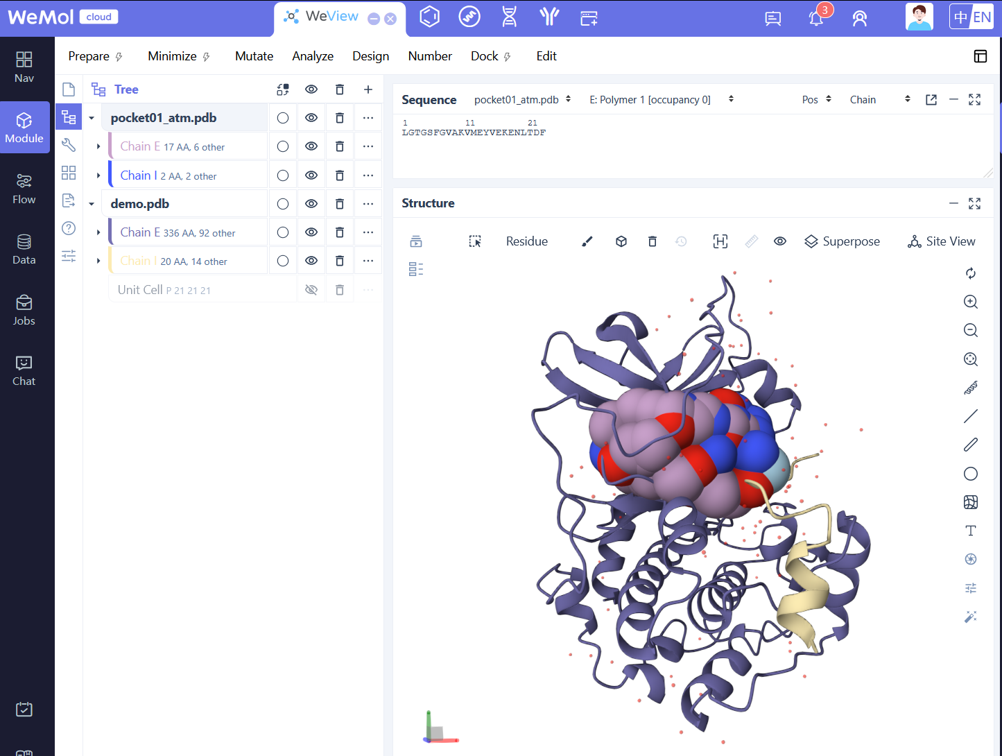
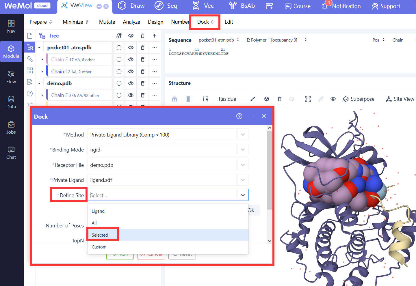
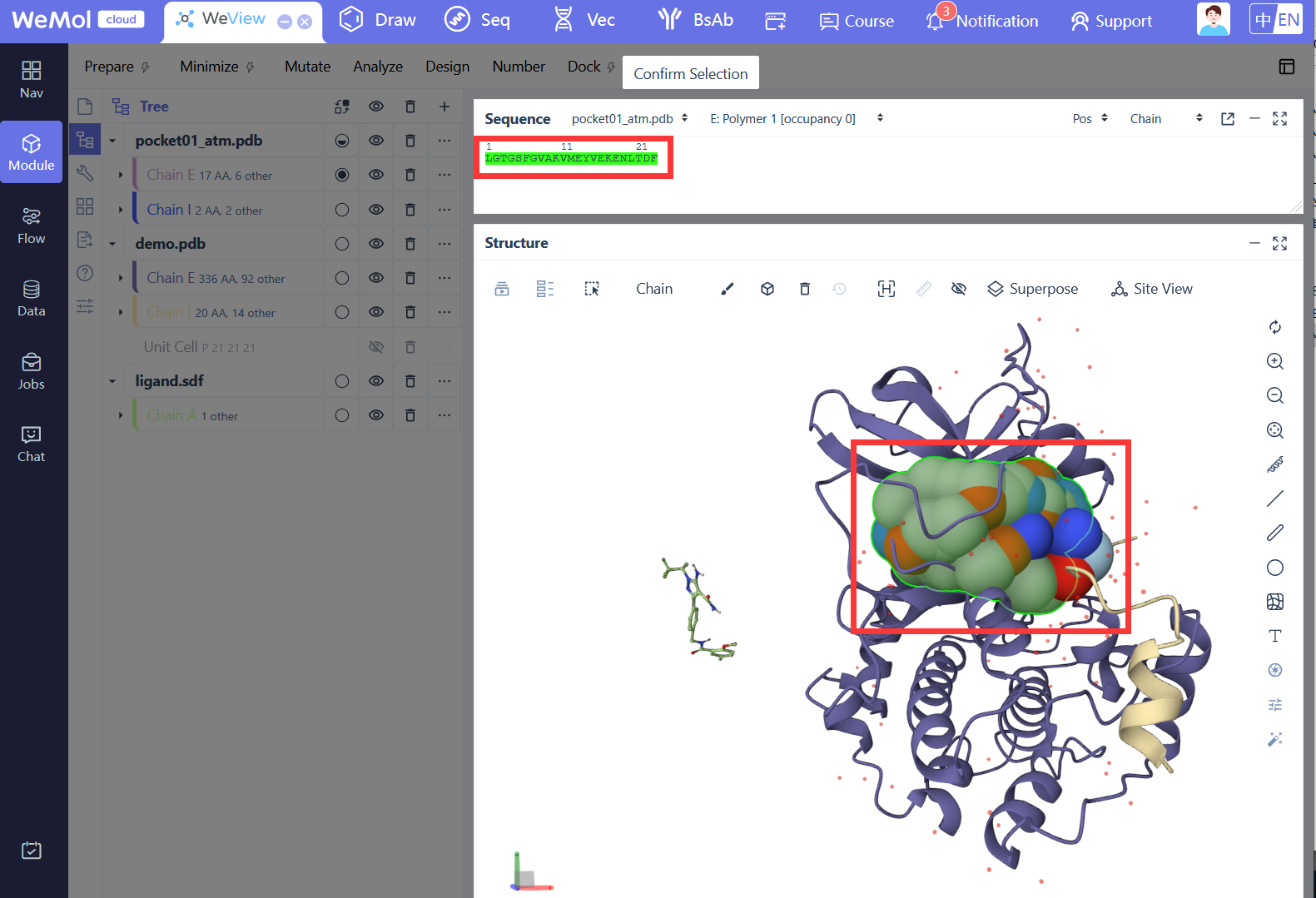
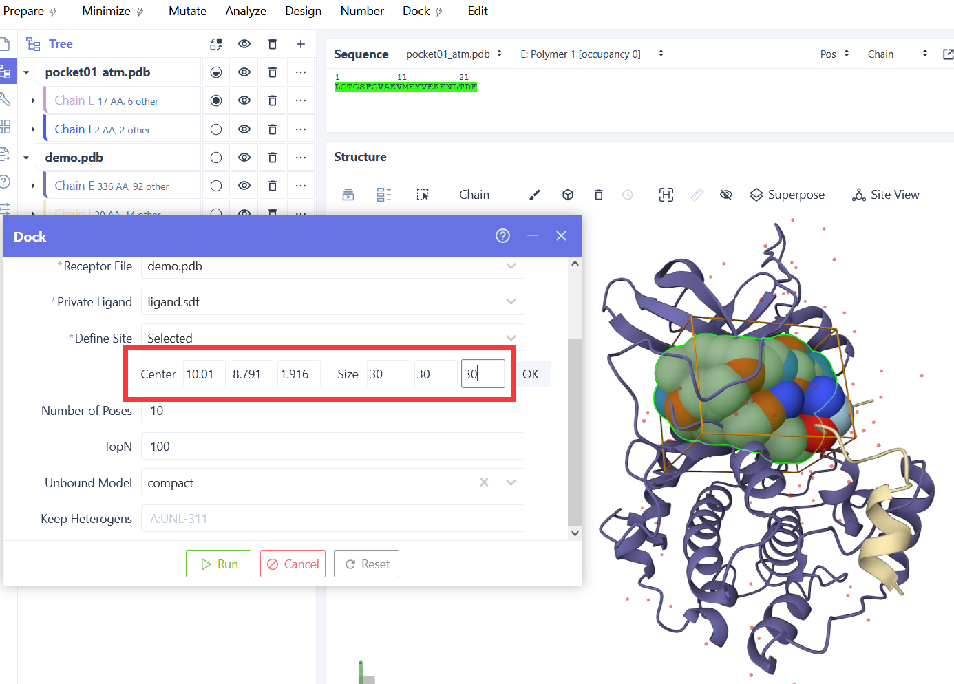
The Pocket Finder module identifies pockets based on geometric and physicochemical properties. Its main function is to quickly and accurately identify potential pockets on the protein surface. Protein pockets (or active sites) are small regions on the protein surface where drug molecules or other small molecules typically bind. Identifying these pockets is crucial for drug design and protein function studies.
The structure file of the protein in PDB format.
The minimum radius of the alpha sphere.
The maximum radius of the alpha sphere.
The distance threshold for the clustering algorithm.
The clustering method used to group Voronoi vertices:
s for single linkage clustering.m for complete linkage clustering.a for average linkage clustering.c for centroid linkage clustering.The distance metric for clustering:
e for Euclidean distance.b for Manhattan distance.The minimum number of alpha spheres per pocket.
The output results include:
| Output File Name | Description |
|---|---|
| pocket_properties.csv | CSV file with pocket information |
| pockets.tar.gz | Compressed archive of PDB files obtained from the protein analysis |
| pocket*_atm.pdb | PDB (atom) file format for each pocket |
The pocket_properties.csv file contains the following information:
| Field Name | Description |
|---|---|
| Pocket order | |
| Score | Comprehensive score of the pocket, considering factors such as size, shape, and hydrophobicity. A higher score indicates a better pocket, more likely to be biologically relevant or suitable for drug binding. |
| Druggability Score | Assesses the potential of the pocket to bind drug molecules. A higher score indicates higher druggability. |
| Total SASA | Total solvent-accessible surface area of the pocket, in square angstroms (Ų); larger SASA indicates the ability to accommodate larger ligand structures. |
| Polar SASA | The polar portion of the total SASA, indicating the surface area accessible to water molecules. Reflects the hydrophilicity of the pocket. |
| Apolar SASA | The apolar portion of the total SASA, indicating the surface area not accessible to water molecules. Reflects the hydrophobicity of the pocket. |
| Volume | The volume of the pocket, in cubic angstroms (ų). A larger volume indicates a larger pocket, capable of accommodating larger ligands or multiple binding sites. |
Restrained Complex Structure Prediction模块基于ColabDock框架实现,ColabDock框架通过整合多种实验限制条件,显著提升了蛋白-蛋白对接预测的准确性。其创新点包括:
ColabDock框架的工作流程分为两个主要阶段:

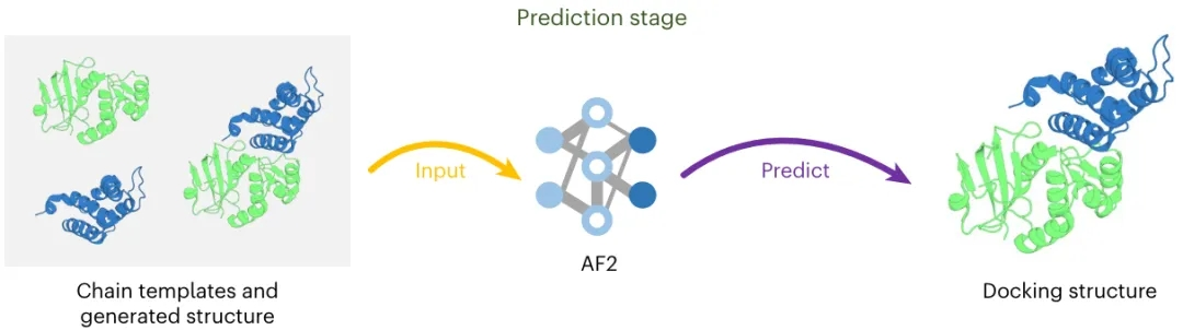
ColabDock主要关注两种类型的约束。第一种约束限制了残基对之间的距离低于某一阈值,属于残基-残基层面的约束(称为1v1约束)。这类约束包括源自交联质谱(XL-MS)的约束。第二种约束定义了在蛋白质表面上可能接触的两组残基之间的约束,但具体的接触信息未知。此类约束属于界面层面的约束(称为MvN约束),典型示例包括多种NMR实验和共价标记(CL)。
ColabDock在模拟约束条件下的性能验证情况如下图所示:
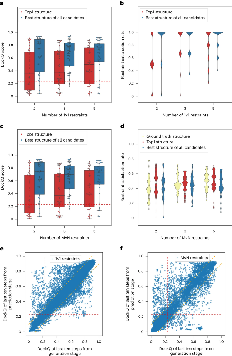
如图a所示,在仅提供两个1v1约束的情况下,81.08%的蛋白质复合物的最大DockQ值超过了0.23,尤其考虑到从这些约束中获取的结构信息相对有限。当提供三到五个约束时,成功率接近100%。如图b所示,对于含有两、三和五对约束的蛋白质复合物,其约束满足率分别为0.55、0.77和0.80。这些结果表明,ColabDock能够高效利用提供的约束来获得高质量的复合物结构。
评估ColabDock在MvN约束下的性能时,先基于上述1v1样本生成了MvN样本。这些样本的挑战性更大,因为MvN约束的模糊性使得多个1v1约束组合可能满足同一组MvN约束。如图c所示,111个样本中有100个预测结构的最大DockQ值超过了0.23。其中,75个样本的top1结构的DockQ值超过0.23。随着约束数量的增加,ColabDock的准确性也相应提高,top1结构的成功率从两个约束时的62.16%上升到三个和五个约束时的70.27%。在预测结构中,约束满足率与实验结构中的比例相似(图d)。这些结果表明,ColabDock同样能够高效利用模糊的约束条件来改善结构预测。
为了评估ColabDock中预测阶段的必要性,在上述1v1和MvN约束实验中,收集了最后十个优化步骤中的结构,大多数优化过程已经收敛。在生成阶段和预测阶段的DockQ值差异较大的情况下(这里定义为大于0.1),预测阶段在69.9%的1v1约束复合物中表现更好(图e),在MvN约束复合物中这一比例为68.8%(图f)。这些结果表明,AF2的能量景观可以帮助优化生成阶段的构象并提高预测的准确性。
ColabDock与传统限制性对接方法比较如下图所示:

基于37个蛋白质复合物的独立基准集。与HADDOCK和ClusPro进行了比较。对于基准集中的每个复合物,采样两、三和五个1v1约束来指导对接,最终生成了111个样本。ColabDock在大多数样本中优于HADDOCK和ClusPro(图a)。ColabDock的平均DockQ值为0.477,而HADDOCK和ClusPro的DockQ值分别为0.287和0.191。无论1v1约束的数量多少,ColabDock在三种方法中均表现最佳(图b)。这些结果表明,ColabDock在稀疏约束条件下有生成可靠结构的潜力,这与验证集的观察结果一致。
为了进一步评估ColabDock在界面级别约束下的表现,作为验证数据集,将上述描述的1v1约束转换为MvN约束。由于ClusPro在111个样本中有7个无法给出预测,将其排除,并对剩余的104个样本进行比较。与1v1约束下的表现相比,由于MvN约束的模糊性,ColabDock、HADDOCK和ClusPro在MvN约束下的表现有所下降,但ColabDock仍然优于其他两种方法(图c)。实验再次表明,无论MvN约束的数量多少,ColabDock在DockQ上均表现最佳(图d)。
实验衍生的约束中常常包含相距较远的残基,作者将其称为“松散约束”。为了测试模型在相关任务中的表现,有意在距离范围为8Å到20Å之间加入了松散约束。对于基准集中的每个复合物,松散约束的数量从1到5不等,而总约束数量固定为5个,共生成了185个样本。排除了9个ClusPro无法处理的样本,并对剩余的176个样本进行了三种方法的比较。结果显示,ColabDock表现最佳,平均DockQ值为0.344,平均α碳原子r.m.s.d.(Cα-r.m.s.d.)为6.55Å(图e)。这些结果表明,ColabDock对约束的质量依赖较低。当与高质量约束结合时,ColabDock能够预测出比其他两种方法更为精确的结构。
抗原抗体复合物预测
抗体-抗原复合物建模一直是一个长期存在的挑战,因为互补决定区(CDRs)的灵活性和缺乏共同进化信号。深度突变扫描(DMS)是一种常用技术,用于确定可能参与抗体-抗原结合的残基。基于一个包含45个复合物的抗体-抗原基准集,通过采样界面上的残基来模拟DMS衍生的约束。预测效果及与传统方法的比较情况如下图所示:
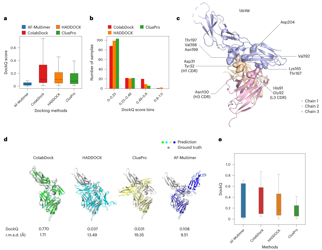
图a所示,ColabDock优于HADDOCK和ClusPro,其平均DockQ值为0.223,平均r.m.s.d.为9.57Å。对于DockQ值大于0.49的样本数量,ColabDock也超过了HADDOCK和ClusPro(图b)。
以1AHW为例:1AHW是一个人类组织因子-抗体(5G9)复合物,参与了血液凝固蛋白酶级联过程。如图c所示,随机从抗体中采样了五个界面残基(轻链的His91和Gly92,重链的Asp31、Tyr32和Asn100),以及从抗原中采样了七个界面残基(Lys165、Thr167、Val192、Thr197、Val198、Asn199和Asp204)。这些在抗体中采样的残基主要分布在L1 CDR、H1 CDR和H3 CDR区域。图d展示了AF-Multimer的预测结构以及三种对接方法的结构。如图e所示,ColabDock捕捉到了大多数界面上的天然接触,其DockQ值为0.770,r.m.s.d.为1.17Å,而其他方法的预测结构与天然构象有较大差异。这一案例研究表明,ColabDock在构象探索和构象排序方面都优于其他两种方法。
初始蛋白复合物结构文件,PDB格式
注:该结构由多条链组成,链与链之间的相对位置可任意放置,无要求。由于显存大小限制,当前最大支持的最终复合物尺寸大小不超过800个残基。
复合物中提取多条链,用于组成最终的复合物结构,链名之间用逗号分隔,如:A,H,L
提取的多条链中指定相对位置固定的每对链,支持定义多对,链名之间用逗号分隔,每行一对,示例如下:
H,L
A,H
表示链H与L之间的相对位置固定,链A与H之间的相对位置固定。
实验限制的距离阈值,表示设置限制的残基间的距离需小于该阈值。默认为8.0 Å,值范围为2.0 Å - 22.0 Å,建议采用默认值。
单个残基之间的限制条件,限制单个残基之间的距离在上述定义的阈值参数内,残基之间用逗号(,)分隔,支持定义多个条件(每行定义一个),示例如下:
A20,H50
A78,L98
该参数表示设置的限制条件有2个:
注意:残基编号为位置编号,即每条链按顺序从1开始进行编号,以下编号规则一致。
单个残基与残基组合之间的限制条件,限制单个残基与多个残基集合中至少一个残基之间的距离在上述定义的阈值参数内,单个残基与残基组合之间用逗号(,)分隔,残基组合内部用分号(;)分隔,可支持定义多个条件(每行定义一个),示例如下:
A10,H60-70;H78;L90
A78,H60-70;L56;L69
A120,L30-L36;H68;H72
2
该参数表示设置的限制条件有3个,分别是:
限制残基间排斥的距离阈值,表示设定的排斥残基间的距离需大于该阈值。默认为8.0 Å,值范围为2.0 Å - 22.0 Å,建议采用默认值。
单个残基间的排斥限制条件,限制单个残基之间的距离需大于上述定义的排斥阈值,残基之间用逗号(,)分隔,可支持定义多个条件(每行定义一个),示例如下:
15,98
60,205
该参数表示设置的排斥限制条件有2个:
输出1st_best.pdb结果文件,为预测得到的最优复合物结构文件。
输出pdbs.tar.gz文件,为预测得到的前5个最优复合物结构文件压缩包。
输出summary.txt文件,包含以下信息:
| 列名 | 说明 |
|---|---|
| pdb | 复合物结构文件名 |
| iptm | 复合物结构的质量好坏评价指标,0-1之间,越接近1表示预测结构的质量越好 |
| # of satisfied restraints | 限制条件的数量,以及预测的复合物结构能满足的条件数量,如:2/2表示有2个限制条件,预测得到的复合物结构都能满足;1/2表示有2个限制条件,但复合物结构只满足了其中1个 |
备注:
可能存在以下个别情况,属正常现象
The module is implemented based on the ColabDock framework, which significantly improves the accuracy of protein-protein docking predictions by integrating a variety of experimental constraints. Its innovations include:
The workflow of the ColabDock framework is divided into two main stages:
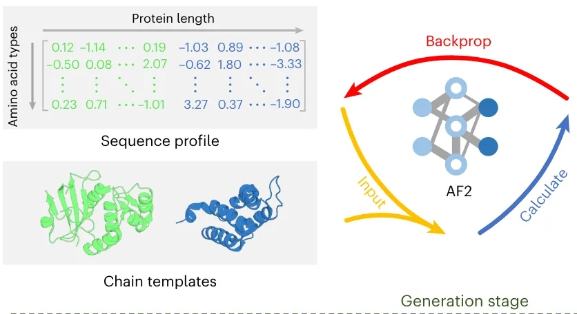

ColabDock focuses on two types of constraints. The first type of constraints restricts the distance between residue pairs to be below a certain threshold and are residue-residue level constraints (called 1v1 constraints). This type of constraints includes constraints derived from cross-linking mass spectrometry (XL-MS). The second type of constraints defines constraints between two groups of residues that may contact on the protein surface, but the specific contact information is unknown. This type of constraints belongs to the interface level constraints (called MvN constraints), and typical examples include various NMR experiments and covalent labeling (CL).
The performance verification of ColabDock under simulation constraints is shown in the following figure:

As shown in Figure a, with only two 1v1 constraints provided, 81.08% of the protein complexes had a maximum DockQ value of more than 0.23, especially considering the relatively limited structural information obtained from these constraints. When three to five constraints were provided, the success rate was close to 100%. As shown in Figure b, for protein complexes containing two, three, and five pairs of constraints, the constraint satisfaction rates were 0.55, 0.77, and 0.80, respectively. These results show that ColabDock can efficiently use the provided constraints to obtain high-quality complex structures.
When evaluating the performance of ColabDock under MvN constraints, MvN samples were first generated based on the above 1v1 samples. These samples are more challenging because the ambiguity of MvN constraints makes it possible for multiple 1v1 constraint combinations to satisfy the same set of MvN constraints. As shown in Figure c, 100 of the 111 samples have a maximum DockQ value of more than 0.23 for the predicted structures. Among them, 75 samples have a DockQ value of more than 0.23 for the top1 structure. As the number of constraints increases, the accuracy of ColabDock also increases accordingly, with the success rate of the top1 structure increasing from 62.16% with two constraints to 70.27% with three and five constraints. In the predicted structures, the constraint satisfaction rate is similar to that in the experimental structures (Figure d). These results show that ColabDock can also effectively use fuzzy constraints to improve structure prediction.
To evaluate the necessity of the prediction stage in ColabDock, structures from the last ten optimization steps were collected in the above 1v1 and MvN constrained experiments, and most of the optimization processes have converged. In cases where the difference in DockQ values between the generation stage and the prediction stage is large (here defined as greater than 0.1), the prediction stage performs better in 69.9% of the 1v1 constrained complexes (Figure e) and in 68.8% of the MvN constrained complexes (Figure f). These results suggest that the energy landscape of AF2 can help optimize conformations in the generation stage and improve the accuracy of predictions.
The comparison between ColabDock and traditional restrictive docking methods is shown in the figure below:
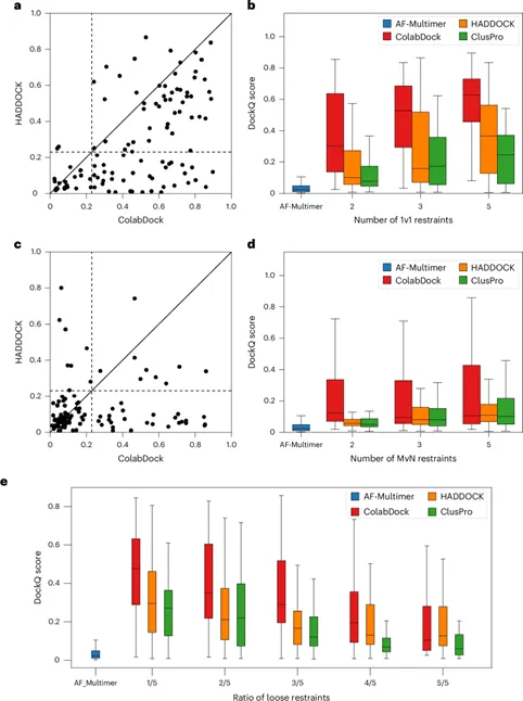
Based on an independent benchmark set of 37 protein complexes. Comparisons were made with HADDOCK and ClusPro. For each complex in the benchmark set, two, three, and five 1v1 constraints were sampled to guide docking, and 111 samples were finally generated. ColabDock outperformed HADDOCK and ClusPro in most samples (Figure a). The average DockQ value of ColabDock was 0.477, while the DockQ values of HADDOCK and ClusPro were 0.287 and 0.191, respectively. Regardless of the number of 1v1 constraints, ColabDock performed best among the three methods (Figure b). These results show that ColabDock has the potential to generate reliable structures under sparse constraints, which is consistent with the observations of the validation set.
To further evaluate the performance of ColabDock under interface-level constraints, the 1v1 constraints described above were converted to MvN constraints as a validation dataset. Since ClusPro could not give predictions for 7 out of 111 samples, it was excluded and the remaining 104 samples were compared. Compared with the performance under 1v1 constraints, the performance of ColabDock, HADDOCK, and ClusPro under MvN constraints declined due to the ambiguity of MvN constraints, but ColabDock still outperformed the other two methods (Figure c). The experiment again shows that ColabDock performs best on DockQ regardless of the number of MvN constraints (Figure d).
Experimentally derived constraints often contain residues that are far apart, which the authors call “loose constraints.” In order to test the performance of the model in related tasks, loose constraints were intentionally added with distances ranging from 8Å to 20Å. For each complex in the benchmark set, the number of loose constraints ranged from 1 to 5, while the total number of constraints was fixed at 5, generating a total of 185 samples. Nine samples that ClusPro could not handle were excluded, and the three methods were compared on the remaining 176 samples. The results showed that ColabDock performed best, with an average DockQ value of 0.344 and an average α-carbon atom r.m.s.d. (Cα-r.m.s.d.) of 6.55Å (Figure e). These results indicate that ColabDock has a low dependence on the quality of constraints. When combined with high-quality constraints, ColabDock is able to predict more accurate structures than the other two methods.
Antigen-antibody complex prediction
Modeling antibody-antigen complexes has been a long-standing challenge due to the flexibility of complementarity determining regions (CDRs) and the lack of co-evolutionary signals. Deep mutational scanning (DMS) is a commonly used technique to identify residues that may be involved in antibody-antigen binding. Based on an antibody-antigen benchmark set of 45 complexes, DMS-derived constraints were simulated by sampling residues on the interface. The prediction results and comparison with traditional methods are shown in the figure below:

As shown in Figure a, ColabDock outperforms HADDOCK and ClusPro, with an average DockQ value of 0.223 and an average r.m.s.d. of 9.57 Å. For the number of samples with a DockQ value greater than 0.49, ColabDock also exceeds HADDOCK and ClusPro (Figure b).
Take 1AHW as an example: 1AHW is a human tissue factor-antibody (5G9) complex that participates in the blood coagulation protease cascade. As shown in Figure c, five interface residues were randomly sampled from the antibody (His91 and Gly92 of the light chain, Asp31, Tyr32 and Asn100 of the heavy chain), and seven interface residues were sampled from the antigen (Lys165, Thr167, Val192, Thr197, Val198, Asn199 and Asp204). These sampled residues in the antibody are mainly distributed in the L1 CDR, H1 CDR and H3 CDR regions. Figure d shows the predicted structure of AF-Multimer and the structures of the three docking methods. As shown in Figure e, ColabDock captures most of the natural contacts on the interface, with a DockQ value of 0.770 and an r.m.s.d. of 1.17Å, while the predicted structures of other methods are quite different from the natural conformation. This case study demonstrates that ColabDock outperforms the other two methods in both conformational exploration and conformational ranking.
Original protein complex structure file, PDB format
Note: This structure consists of multiple chains, and the relative positions between chains can be placed arbitrarily. Due to the limitation of GPU memory, the current maximum supported final complex size does not exceed 800 residues.
Multiple chains are extracted from the original complex to form the final complex structure. The chain names are separated by commas, such as: A,H,L
Specify each pair of chains with fixed relative positions among the extracted multiple chains. Multiple pairs can be defined. Chain names are separated by comma, with one pair per line. The example is as follows:
H,L
A,H
It means that the relative position between chains H and L is fixed, and the relative position between chains A and H is fixed.
The distance threshold of the experimental restraint, which means that the distance between the residues to set the restraint must be less than this threshold. The default value is 8.0 Å, and the value range is 2.0 Å - 22.0 Å. The default value is recommended.
Restrictions between single residues. Limit the distance between single residues to the threshold parameters defined above. Residues are separated by commas. Multiple conditions can be defined (one per line). The following is an example:
A20,H50
A78,L98
This parameter indicates that there are two restrictions set:
The restriction conditions between a single residue and a residue combination limit the distance between a single residue and at least one residue in a set of multiple residues to be within the threshold parameters defined above. Single residues and residue combinations are separated by commas, and residue combinations are separated by semicolons. Multiple conditions can be defined (one per line). The following is an example:
A10,H60-70;H78;L90
A78,H60-70;L56;L69
A120,L30-L36;H68;H72
2
This parameter indicates that there are three restrictions set, namely:
The distance threshold for limiting the repulsion between residues, indicating that the distance between the set repulsive residues must be greater than this threshold. The default value is 8.0 Å, and the value range is 2.0 Å - 22.0 Å. It is recommended to use the default value.
The exclusion constraint between single residues requires the distance between single residues to be greater than the exclusion threshold defined above. Residues are separated by comma. Multiple conditions can be defined (one per line). The following is an example:
15,98
60,205
This parameter indicates that there are two exclusion constraints set:
‘1st_best.pdb’ file, which is the predicted optimal complex structure file.
‘pdbs.tar.gz’ file, which is the compressed package of the top 5 predicted optimal complex structure files.
‘summary.txt’ file, which contains the following information:
| Fields | Introduction |
|---|---|
| pdb | File name of complex structure |
| iptm | An evaluation index of the quality of the complex structure, between 0 and 1, the closer to 1, the better the quality of the predicted structure |
| # of satisfied restraints | The total number of constraints and the number of constraints that the predicted complex structure can satisfy. For example, 2/2 means that there are 2 constraints and the predicted complex structure can satisfy them all; 1/2 means that there are 2 constraints, but the complex structure only satisfies one of them. |
Note:
The following individual cases may exist, which are normal:
Germline Blast模块基于IgBlastp实现,通过氨基酸序列比对从IMGT reference sequences数据库中搜索与目标抗体序列最接近的同源模板,输出对应的模板序列以及序列一致性等信息。数据库中默认检索的序列类型为:IMGT V genes(F+ORF+in-frame P)。
抗体的序列文件,FASTA格式。
抗体编号类型:kabat和imgt
输出同源性最高的N条序列,默认值为10。
序列所属物种:Human,Mouse,Rat,Rabbit,Rhesus_Monkey,Alpaca,默认值为Human。
| 输出参数 | 输出文件名称 | 说明 |
|---|---|---|
| Hits Sequence | hits.fasta | 包含同源性最高的n条序列的序列文件 |
| Result | result.csv | 包含找到的Germline序列以及序列的一致性信息 |
| Alignment Summary | align_info_top_germline.csv | 包含查询序列与同源性最高的Germline V基因序列的比对信息 |
The Germline Blast module is based on IgBlastp and searches for the most homologous templates to the target antibody sequence from the IMGT reference sequences database through sequence alignment. It outputs the corresponding template sequences and sequence identity information. The default sequence types searched in the database are: IMGT V genes (F+ORF+in-frame P).
The antibody sequence file in FASTA format.
The antibody numbering scheme: kabat and imgt.
The number of top homologous sequences to output, with a default value of 10.
The species of the sequence: Human, Mouse, Rat, Rabbit, Rhesus_Monkey, Alpaca,with the default value being Human.
| Output Parameter | Output File Name | Description |
|---|---|---|
| Hits Sequence | hits.fasta | A sequence file containing the top N homologous sequences |
| Result | result.csv | Contains the identified germline sequences and sequence identity information |
| Alignment Summary | align_info_top_germline.csv | Contains alignment information between the query sequence and the top homologous germline V gene sequences |
Mutation Energy of Stability (ThermoMPNN)模块基于ThermoMPNN模型实现,此深度神经网络模型可根据蛋白初始结构,预测单点突变对应的稳定性变化。模型使用从ProteinMPNN(一种深度神经网络模型,可根据蛋白质的三维结构预测其氨基酸序列)中提取的结构特征,在已建立的基准数据集上实现了优秀的预测性能。通常认为,ddG < -0.5 kcal/mol 可能是一个有利于稳定性的突变。ThermoMPNN 在 Fireprot(HF)数据集上的正预测值为 56%(34/61 个预测为稳定的突变),在 Megascale 数据集上为 46%(1,312/2,852)。
模型架构与数据集分析如下图所示:

模型预测效果与其他方法效果比较见下图:

蛋白的结构文件,PDB格式,支持单体或复合物结构
用于稳定性突变分析的链名称,仅支持单链,如:A
抗体编号规则,支持Kabat, Chothia和IMGT,默认为Kabat。
指定输出能量最优的前N个突变对应的序列,默认为100。
输出文件名称,默认pred_res.csv。
输出TopN对应的突变链的序列,默认为mutant_seqs.fasta。
输出TopN对应的复合物序列,复合物中各链之间用分号:分隔(Boltz2结构预测的批量模式),默认为mutant_seqs_complex.fasta。
输出result.csv结果文件,包含以下信息:
| 列名 | 说明 |
|---|---|
| Chain | 链名称,如:'A’表示A链 |
| Mutation | 单点突变信息,如:'G1A’表示序列编号为1的残基甘氨酸G,突变为丙氨酸A,序列编号从1开始按顺序编号(非PDB文件中的残基序号) |
| ddG_pred | 突变对应的能量变化,负值表示体系能量较低,体系变得更稳定。负得越多表示稳定性提升越多。ddG < -0.5 kcal/mol 可能是一个有利于稳定性的突变 |
输出TopN对应的突变链的序列mutant_seqs.fasta。
输出TopN对应的复合物序列,复合物中各链之间用冒号:分隔(Boltz2结构预测的批量模式)mutant_seqs_complex.fasta。
The Mutation Energy of Stability (ThermoMPNN) module is based on the ThermoMPNN model. This deep neural network model predicts the stability changes corresponding to single-point mutations based on the initial structure of the protein. The model uses structural features extracted from ProteinMPNN (a deep neural network model that predicts amino acid sequences based on the three-dimensional structure of proteins) and has achieved excellent predictive performance on established benchmark datasets.If we consider a ΔΔG° < -0.5 kcal/mol to indicate a stabilizing mutation, ThermoMPNN achieves a PPV of 56% (34/61 predicted stabilizing mutations) on the Fireprot (HF) dataset and 46% (1,312/2,852) on the Megascale dataset.
The model architecture and dataset analysis are shown in the figure below:
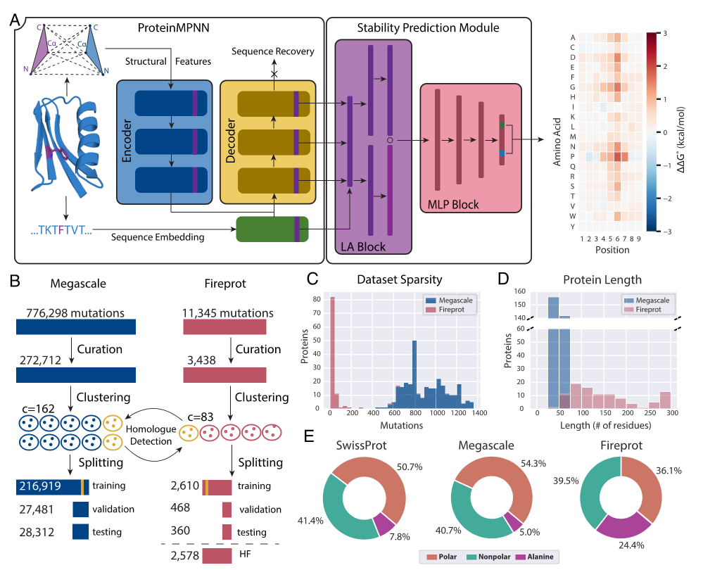
The comparison of the model’s predictive performance with other methods is shown in the figure below:
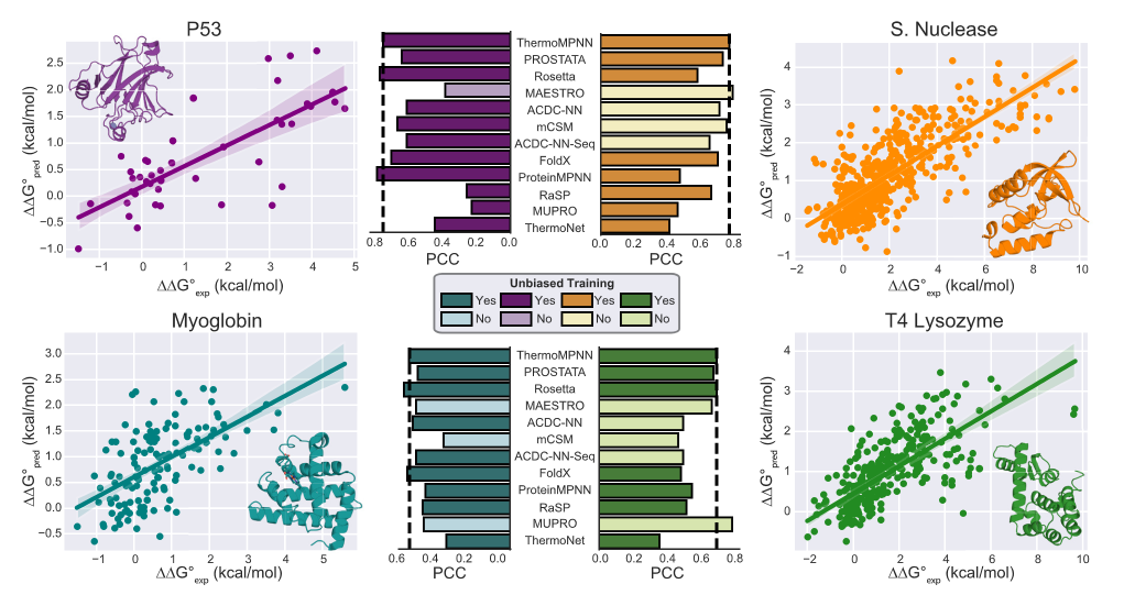
The structure file of the protein in PDB format, supporting monomer or complex structures.
The name of the chain for stability mutation analysis, supporting only single chains, e.g., A.
Antibody numbering schemes, supporting Kabat, Chothia, and IMGT. The default scheme is Kabat.
Specify the sequences corresponding to the top N mutations with the optimal energy. The default value is 100.
Output file name, pred_res.csv is the default.
Output the sequences of the mutation chains corresponding to TopN.
Output the sequences of the complexes corresponding to TopN. The chains within the complexes are separated by semicolons (;) (for batch mode structure prediction by Boltz2).
The output result.csv file contains the following information:
| Column Name | Description |
|---|---|
| Chain | The name of the chain, e.g., ‘A’ for chain A |
| Mutation | Single-point mutation information, e.g., ‘G1A’ means the residue glycine G at sequence number 1 is mutated to alanine A. The sequence number starts from 1 in order (not the residue number in the PDB file) |
| ddG_pred | The energy change corresponding to the mutation. A negative value indicates lower system energy and increased stability. The more negative, the greater the stability improvement. ddG < -0.5 kcal/mol may indicate a stabilizing mutation |
Output the sequences of the mutation chains corresponding to TopN. mutant_seqs.fasta
Output the sequences of the complexes corresponding to TopN. The chains within the complexes are separated by : (for batch mode structure prediction by Boltz2). mutant_seqs_complex.fasta
Homology Tree模块用于生成同源性进化树。
蛋白序列文件,FASTA格式。
输出结果包括:
| 输出文件名称 | 说明 |
|---|---|
| alignment.fasta | 按树结构顺序输出的叠合后的序列文件的FASTA文件 |
| tree.png | 多重序列树结构图片 |
The Homology Tree module is used to generate homologous evolutionary trees.
Protein sequence file in FASTA format.
The output includes:
| Output File Name | Description |
|---|---|
| alignment.fasta | FASTA file of the superimposed sequence of files output in order of tree structure. |
| tree.png | Tree structure picture of multiple sequence |
Structure Evolution模块基于ESMIF模型实现,ESMIF逆折叠模型旨在根据蛋白质主链原子坐标预测蛋白序列。该模型使用AlphaFold2预测的1200万个蛋白质结构进行训练,包含不变几何输入处理层,随后是一个序列到序列的Transformer,对于在结构上保持不变的主干序列实现51%的本地序列恢复率,对于埋藏残基实现72%的恢复率。该模型还经过跨度屏蔽训练,能够容忍缺失的主链坐标,因此可以预测部分被屏蔽结构的序列。该模块既可以用于亲和力成熟,也可以用于稳定性优化。
蛋白的结构文件,PDB格式,支持单体或复合物结构
用于进化分析的链名称,仅支持单链,默认为A链
指定目标链中的多个残基,进行多点突变分析。使用残基位置编号(从1开始),多个残基用逗号分隔,指定残基范围用横杠符号。如:“3,10,24-30”表示目标链上的第3、第10与第24至30号残基,参与多点突变分析。
备注:如不设置该参数,表示采用目标链的全长序列进行突变分析。
指定突变点最小数目,默认值为1,表示从单点突变开始进行突变分析。如设置为2,表示从两点组合突变开始进行突变分析。
指定突变点最大数目,默认值为3,表示至多进行三点组合突变。如设置为2时,表示最多进行两个点的多点组合突变。
指定参与多点突变分析的每个残基,其最大的替换数目,默认为5,表示每个残基最多突变为5种不同的其他残基。
备注:理论上,每种残基可以突变为其他19种天然残基,但因多点突变可能引起的组合爆炸,这里我们限制了最大替换数目。每个残基具体替换的其他残基类别,会根据ESMIF模型给出的该位置残基的概率分布,优先选择概率高的残基类别。
输出CSV文件名称,包含了突变以及对应的突变的可能性。
抗体编号规则,支持Kabat, Chothia和IMGT,默认为Kabat。
指定输出评分最优的前N个突变对应的序列,默认为100。
输出TopN对应的突变链的序列,默认为mutant_seqs.fasta。
输出TopN对应的复合物序列,复合物中各链之间用冒号:分隔(Boltz2结构预测的批量模式),默认为mutant_seqs_complex.fasta。
输出结果文件,包含以下信息:
| 列名 | 说明 |
|---|---|
| Mutation | 单点突变信息,如:'WT’表示野生型原序列,'G1A’表示序列编号为1的残基甘氨酸G,突变为丙氨酸A,序列编号从1开始按顺序编号(非PDB文件中的残基序号) |
| Log_likelihood | 输入结构的全部序列对应的模型预测概率对数值,越大表示该突变序列越好 |
| Log_likelihood_target_chain | 输入结构的目标链序列(对应参数Target Chain)对应的模型预测概率对数值,越大表示该突变序列越好 |
| Interface | 用于标识残基是否位于分子接触界面。留空表示不进行界面计算;取值为 0 表示该残基不属于接触界面;取值为 1 表示该残基属于接触界面 |
| Domain(Chothia) | 当输入为抗体序列或结构时,根据 Chothia 定义输出对应的FR(Framework Region)和CDR(Complementarity-Determining Region)区域注释 |
| Likelihood(ESMIF) | Log_likelihood列进行去log,同时减去WT数值后的值,其数值大于0表示该突变优于WT,越大越好。 |
| Likelihood_target_chain(ESMIF) | Log_likelihood_target_chain列进行去log,同时减去WT数值后的值,其数值大于0表示该突变优于WT,越大越好。 |
注释:当输入结构为单链时,Log_likelihood与Log_likelihood_target_chain数值一致。当输入结构为复合物时,Log_likelihood对应的是复合物的全部序列的概率值,Log_likelihood_target_chain对应的是复合物中目标链序列(参数Target Chain)对应的概率值。
输出TopN对应的突变链的序列mutant_seqs.fasta。
输出TopN对应的复合物序列mutant_seqs_complex.fasta,复合物中各链之间用冒号:分隔(Boltz2结构预测的批量模式)。
The Structure Evolution module is based on the ESMIF model and is used for structure-based single-point advantageous mutation analysis. The ESMIF inverse folding model aims to predict protein sequences from the coordinates of protein backbone atoms. This model is trained on 12 million protein structures predicted by AlphaFold2 and includes invariant geometric input processing layers followed by a sequence-to-sequence Transformer. It achieves a 51% local sequence recovery rate for backbone sequences that remain structurally invariant and a 72% recovery rate for buried residues. The model is also trained with span masking, allowing it to tolerate missing backbone coordinates and predict sequences for partially masked structures. This module can be used for both affinity maturation and stability optimization.
The structural file of the protein in PDB format, supporting both monomer and complex structures.
The name of the chain used for evolutionary analysis. Only single chains are supported. After uploading the structural file, you can select a chain name from the list of chains.
Multiple residues in the chain were labeled for multi-point mutation analysis. Use a residue location number (starting at 1), multiple residues are separated by commas, and a delimiter is used to specify the residue range. For example, “3,10,24-30” indicates residues 3,10, and 24 to 30 on the target chain, which participate in multipoint mutation analysis.
Specifies the minimum number of mutation points, the default is 1, indicating that mutation analysis starts with single mutation. If the value is set to 2, it indicates that the mutation analysis starts from the two-point mutation.
Specifies the maximum number of mutation points, the default is 3, indicating that at most three points of combination mutation can be made. If the value is set to 2, it indicates that a maximum of two points of combination mutation can be performed.
Specifies the maximum number of substitutions for each residue participating in multipoint mutation analysis, which defaults to 5, meaning that each residue mutates up to 5 different other residues.
Output CSV file containing the mutations and corresponding probabilities.
Antibody numbering schemes, supporting Kabat, Chothia, and IMGT.
The default scheme is Kabat.
Designate the sequences corresponding to the top N mutations with the best scores, with a default value of 100.
Output the sequences of the mutation chains corresponding to TopN, with a default file name of mutant_seqs.fasta.
Output the sequences of the complexes corresponding to TopN. The chains within the complex are separated by colons(:) (for batch mode of Boltz2 structure prediction), with a default file name of mutant_seqs_complex.fasta.
The output file contains the following information:
| Column Name | Description |
|---|---|
| Mutation | Single-point mutation information, e.g., ‘WT’ represents the wild-type original sequence, ‘G1A’ indicates that the residue glycine (G) at sequence position 1 is mutated to alanine (A). Sequence numbering starts from 1 in order (not the residue number in the PDB file). |
| Log_likelihood | The log value of the predicted probability of the sequences of input structure by the model. The higher the value, the better the mutated sequence. If this value is greater than the corresponding value of WT, it indicates that the mutation is advantageous. |
| Log_likelihood_target_chain | The log-likelihood value of the model’s predicted probability corresponding to the target chain sequence of the input structure (parameter Target Chain). The higher the value, the better the mutated sequence. If this value is greater than the corresponding value of WT, it indicates that the mutation is advantageous. |
| Interface | Indicates whether a residue is part of a molecular interaction interface. Leaving the field empty disables interface calculation; a value of 0 denotes a non-interface residue, whereas 1 denotes an interface residue. |
| Domain(Chothia) | When the input is an antibody sequence or structure, this field outputs annotations of FR (Framework Regions) and CDR (Complementarity-Determining Regions) according to the Chothia numbering scheme |
| Likelihood(ESMIF) | Exponentiated log-likelihood value minus the WT value. Values greater than 0 indicate the mutation is superior to WT; larger values are better. |
| Likelihood_target_chain(ESMIF) | Exponentiated log_likelihood_target_chain value minus the WT value. Values greater than 0 indicate the mutation is superior to WT; larger values are better. |
Output the sequences of the mutation chains corresponding to TopN mutant_seqs.fasta.
Output the sequences of the complexes corresponding to TopN mutant_seqs_complex.fasta. The chains within the complex are separated by colons(:) (for batch mode of Boltz2 structure prediction) .
Note: When the input structure is a single chain, the value of Log_likelihood is consistent with that of Log_likelihood_target_chain. When the input structure is a complex, Log_likelihood corresponds to the probability value of the entire sequence of the complex, and Log_likelihood_target_chain corresponds to the probability value of the target chain sequence (parameter Target Chain) in the complex.
进行蛋白或核酸的结构比对,支持单体或异源寡聚体。使用US-align工具实现。输出TM-score,RMSD等衡量结构相似性的指标。可比对序列不一致的蛋白或核酸结构。
用于结构比对的第一个结构,支持批量结构,批量格式支持:.zip,.tar,.tar.gz,.tgz,.tar.bz2,.tbz2,.tar.xz,.txz ,当前最大支持1000个结构。
用于结构比对的第二个结构,定义同上。
注意:结构比对会将PDB1中的所有结构与PDB2中的所有结构进行两两比对。
指定结构中进行叠合的链,格式为:文件名:链名1,链名2,每行定义一个结构的链信息。示例如下:
结构名称1:A,B
结构名称2:C,D
表示结构1中的A链与结构2中的C链进行叠合比对,B链与D链进行叠合比对。
为了方便统一定义所有结构的叠合链,支持只输入逗号分隔的链名列表或链顺序列表,如:A,B或者1,2,前者表示所有结构中都用A,B链进行叠合,后者表示所有结构中都使用第一和第二条链进行叠合。
若结构1与结构2共有链C,输入共有链名(如:C)或其位置索引(如:3)。若抗原为第三条链,填写C或3均可将其作为基准进行叠合。
注意:结构比对会将PDB1中的所有结构与PDB2中的所有结构进行两两比对。
比对结果文件,CSV格式,默认为align_results.csv。
叠合的结构文件,默认为aligned_pdbs.tar.gz
输出结构比对结果文件align_results.csv,包含信息如下:
| 列名 | Description |
|---|---|
| PDB1 | 第一个结构的名称 |
| PDB2 | 第二个结构的名称 |
| TM-score (Norm by Length of PDB1) | TM-score是用于评估蛋白质结构相似性的指标。范围在0到1之间:>0.5:通常认为两个蛋白质具有相同的折叠(同一家族);<0.3:表示结构随机无关(即使长度相同)。这里Norm by Length of PDB1表示将PDB1结构作为参考结构进行归一化的打分。 |
| TM-score (Norm by Length of PDB2) | 表示将PDB2结构作为参考结构进行归一化的TM-score |
| TM-score (Average) | 以上两种归一化 TM-score 的平均值,用于给出两种结构整体相似性的综合评估。 |
| RMSD | 两个结构的骨架结构RMSD值 |
| Aligned_length | 两个结构比对过程中会进行叠合,叠合后的重叠长度(残基数量)。 |
| Sequence_identity | 叠合部分的序列一致性 |
| Aligned_structure | 叠合后的结构名称 |
Performs structural alignment of proteins or nucleic acids, supporting both monomers and hetero-oligomers. The alignment is implemented using the US-align tool and outputs metrics such as TM-score and RMSD to quantify structural similarity.
It supports alignment between protein or nucleic acid structures with non-identical sequences.
The first structure used for alignment. Batch processing is supported with the following archive formats: .zip, .tar, .tar.gz, .tgz, .tar.bz2, .tbz2, .tar.xz, .txz.
Up to 1000 structures are supported at a time.
The second structure used for alignment, defined in the same way as PDB1.
Note: Structural comparison will perform pairwise alignments between all structures in PDB1 and all structures in PDB2.
Specify the chains used for structural superposition. The format is:
structure_name:chain1,chain2, where each line defines the chain information for one structure. Examples:
structure1:A,B
structure2:C,D
This means that chain A in structure 1 is aligned with chain C in structure 2, and chain B is aligned with chain D.
For convenience, to apply a unified chain mapping to all structures, you may also provide only a comma-separated list of chain names or chain indices, such as A,B or 1,2.
A,B indicates that chains A and B are used for alignment in all structures.1,2 indicates that the first and second chains are used for alignment in all structures.Specify the shared chain for alignment by entering its Chain ID (e.g., C) or Positional Index (e.g., 3). For example, if the antigen is the third chain, entering C or 3 will set it as the reference for superposition.
Note: Structural alignment performs pairwise comparisons between all structures in PDB1 and all structures in PDB2.
The alignment results are written to a CSV file, named align_results.csv by default.
The aligned structure files. The default output is aligned_pdbs.tar.gz.
The output file align_results.csv contains the following information:
| Field | Description |
|---|---|
| PDB1 | Name of the first structure |
| PDB2 | Name of the second structure |
| TM-score (Norm by Length of PDB1) | TM-score is a measure of structural similarity between proteins. It ranges from 0 to 1: values >0.5 usually indicate the same fold (same family); values <0.3 indicate random or unrelated structures (even with similar lengths). “Norm by Length of PDB1” means normalization is based on the length of PDB1. |
| TM-score (Norm by Length of PDB2) | TM-score normalized by the length of PDB2 |
| TM-score (Average) | The average of the two normalized TM-scores, providing an overall and balanced assessment of the structural similarity between the two proteins. |
| RMSD | RMSD value between the backbones of the two structures |
| Aligned_length | The number of residues that overlap after structural superposition |
| Sequence_identity | Sequence identity of the aligned region |
| Aligned_structure | Name of the superimposed structure |
Antibody Design (MEAN)模块基于MEAN模型实现,该模型采用多通道等变图注意力网络,可用于设计CDR的一维序列和三维结构。具体而言,MEAN 通过导入额外的结构信息(包括目标抗原和抗体的轻链)将抗体设计公式化为条件图翻译问题。然后,MEAN重新采用 E(3)-等变消息传递以及提出的注意机制来更好地捕捉不同结构信息之间的几何相关性。最后,它通过多轮渐进式全景模式输出一维序列和三维结构,与以前的自回归方法相比,它具有更高的效率和精度。MEAN在序列和结构建模、抗原结合CDR设计和结合亲和力优化方面明显超越了届时最优模型。具体而言,抗原结合CDR设计相对于基线模型改进约为23%,亲和力优化相对于基线模型改进约为34%。
MEAN模型架构如下图所示:
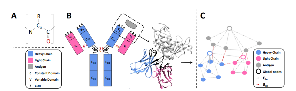

抗体-抗原复合物结构或抗体结构(建议采用复合物结构,设计效果更佳),PDB格式
指定结构中的抗体重链名称,默认值为H,注意如果上传的结构中抗体重链命名非H,请修改该参数为相应的链名
指定结构中的抗体轻链名称,默认值为L,注意如果上传的结构中抗体轻链命名非L,请修改该参数为相应的链名
设计模式,有两种设计模式:CDR-H3设计与亲和力优化(Optimized)
亲和力优化中,生成的结构数量,默认值为100
指定输出亲和力最优的前N个突变对应的序列,默认为100。
输出TopN对应的突变链的序列,默认为mutant_seqs.fasta。
输出TopN对应的复合物序列,复合物中各链之间用冒号:分隔(Boltz2结构预测的批量模式),默认为mutant_seqs_complex.fasta。
输出结果包括:
| 输出文件名称 | 说明 |
|---|---|
| cdrs.txt文件 | 包含设计的CDR-H3序列 |
| design.pdb文件 | 设计后的复合物结构文件,注意抗体结构只保留Fv区域 |
输出结果包括:
| 输出文件名称 | 说明 |
|---|---|
| ddg_scores.txt文件 | 优化后结构与原结构的亲和力差异评分 |
| opt_best.pdb文件 | 亲和力最优结构文件,注意抗体结构只保留Fv区域 |
| log.txt | 亲和力优化文件日志 |
| opt.zip | 优化后的多个结构的压缩文件 |
其中,ddg_scores.txt文件,包含信息如下:
| 列名 | 说明 |
|---|---|
| Name | 结构名称 |
| ddG | 与原结构的亲和力差异评分ddG,单位为kcal/mol,数值为负时表示亲和力有提升,负得越多表示亲和力提升越好 |
输出TopN对应的突变链的序列mutant_seqs.fasta。
输出TopN对应的复合物序列mutant_seqs_complex.fasta,复合物中各链之间用冒号:分隔(Boltz2结构预测的批量模式)。
The Antibody Design (MEAN) module is implemented based on the MEAN model, which employs a multi-channel equivariant graph attention network for designing the one-dimensional sequence and three-dimensional structure of the CDR (Complementarity-Determining Region). Specifically, MEAN formulates antibody design as a conditional graph translation problem by incorporating additional structural information, including the target antigen and the light chain of the antibody. MEAN then re-adopts E(3)-equivariant message passing and the proposed attention mechanism to better capture the geometric correlations between different structural information. Finally, it outputs the one-dimensional sequence and three-dimensional structure through multiple rounds of progressive panoramic mode. Compared to previous autoregressive methods, it has higher efficiency and accuracy. MEAN significantly outperforms the then state-of-the-art models in sequence and structure modeling, antigen-binding CDR design, and binding affinity optimization. Specifically, antigen-binding CDR design improves by approximately 23% over baseline models, and affinity optimization improves by approximately 34% over baseline models.
The MEAN model architecture is shown in the figure below:
The structure of the antibody-antigen complex or the antibody structure (the complex structure is recommended for better design results), in PDB format.
Specify the name of the antibody heavy chain in the structure, the default value is H. Note that if the antibody heavy chain in the uploaded structure is not named H, please modify this parameter to the corresponding chain name.
Specify the name of the antibody light chain in the structure, the default value is L. Note that if the antibody light chain in the uploaded structure is not named L, please modify this parameter to the corresponding chain name.
Design mode, there are two design modes: CDR-H3 design and affinity optimization (Optimized).
In affinity optimization, the number of generated structures, the default value is 100.
Specify the sequences corresponding to the top N mutations with the optimal energy. The default value is 100.
Output the sequences of the mutation chains corresponding to TopN. Default is mutant_seqs.fasta.
Output the sequences of the complexes corresponding to TopN. The chains within the complexes are separated by colon(:) (for batch mode structure prediction by Boltz2). Default is mutant_seqs_complex.fasta.
The output results include:
| Output File Name | Description |
|---|---|
| cdrs.txt | Contains the designed CDR-H3 sequences |
| design.pdb | The designed complex structure file, note that only the Fv region of the antibody structure is retained |
The output results include:
| Output File Name | Description |
|---|---|
| ddg_scores.txt | Affinity difference scores between the optimized structure and the original structure |
| opt_best.pdb | The structure file with the best affinity, note that only the Fv region of the antibody structure is retained |
| log.txt | Affinity optimization log file |
| opt.zip | Compressed file of multiple optimized structures |
The ddg_scores.txt file contains the following information:
| Column Name | Description |
|---|---|
| Name | Structure name |
| ddG | Affinity difference score ddG with the original structure, in kcal/mol. A negative value indicates an improvement in affinity, and the more negative, the better the improvement in affinity |
Output the sequences of the mutation chains corresponding to TopN mutant_seqs.fasta.
Output the sequences of the complexes corresponding to TopN mutant_seqs_complex.fasta. The chains within the complex are separated by colons(:) (for batch mode of Boltz2 structure prediction) .
Venn Diagram Plot是一个制作韦恩图(Venn diagram)模块,常用于比较两个集合的重叠区域以及提取公共部分内容。用于中药网络药理学分析中提取中药成分预测靶点与疾病相关靶点的交集。
集合A文件,TXT格式,每行一个元素。
集合B文件,TXT格式,每行一个元素。
作图时显示的图例,逗号分割,如:set A,set B
比较时是否大小写敏感:
Yes:区分大小写比较
No:不区分大小写比较
输出包含交集部分内容的文件名称,默认为intersection.txt
输出韦恩图文件venn_diagram.png以及交集部分内容的文本文件intersection.txt
The Venn Diagram Plot module is used to create Venn diagrams, which are commonly utilized to compare the overlapping regions of two sets and extract the common elements. This is particularly useful in traditional Chinese medicine network pharmacology analysis for identifying the intersection of predicted targets of herbal components and disease-related targets.
The file for set A, in TXT format, with one element per line.
The file for set B, in TXT format, with one element per line.
The labels to be displayed in the diagram, separated by commas, e.g., set A,set B.
Whether the comparison is case-sensitive:
The name of the output file containing the intersection elements, default is intersection.txt.
The output includes a Venn diagram file named venn_diagram.png and a text file containing the intersection elements named intersection.txt.

检索成对的蛋白-蛋白相互作用(PPI),基于STRING蛋白互作网络数据库,包含蛋白直接物理作用的互作关系以及间接作用的互作关系。
蛋白名称列表文件,TXT格式,一行一个蛋白名称
蛋白-蛋白关联性打分的截断值,0~1之间,只导出combined_score为截断值以上的蛋白-蛋白相互作用数据。
是否输出相关蛋白;
Yes:代表输出与输入蛋白相关的蛋白
No:代表只输出输入蛋白之间存在的相互作用
输出蛋白-蛋白相互作用文件string_interactions.tsv,每一列说明如下:
| 列名 | 说明 |
|---|---|
| node1 | 节点1的蛋白名称 |
| node2 | 节点2的蛋白名称 |
| node1_string_id | 节点1在STRING数据库中标准ID |
| node2_string_id | 节点1在STRING数据库中标准ID |
| neighborhood_on_chromosome | 基于基因组邻近性预测的相互作用得分。 |
| gene_fusion | 基于基因融合事件预测的相互作用得分。 |
| phylogenetic_cooccurrence | 基于共同出现(共现性)预测的相互作用得分。 |
| homology | 蛋白之间的同源性。 |
| coexpression | 基于共同表达(共表达)预测的相互作用得分。 |
| experimentally_determined_interaction | 基于实验数据(例如,酵母双杂交实验)预测的相互作用得分。 |
| database_annotated | 基于已知数据库信息预测的相互作用得分。 |
| automated_textmining | 基于文本挖掘预测的相互作用得分。 |
| combined_score | 综合所有上述信息计算得到的综合得分。 |
Protein-Protein Interaction (STRING) is a module based on the STRING database for extracting protein interaction data. STRING is a protein interaction network database that includes both direct physical interactions and indirect functional associations between proteins.
A file containing a list of protein names, in TXT format, with one protein name per line.
A cutoff value for the protein-protein association score, ranging from 0 to 1. Only protein-protein interactions with a combined score above this cutoff will be exported.
Whether to output related proteins:
The output is a protein-protein interaction file named string_interactions.tsv. Each column is described as follows:
| Column Name | Description |
|---|---|
| node1 | Protein name of node 1 |
| node2 | Protein name of node 2 |
| node1_string_id | Standard STRING ID for node 1 |
| node2_string_id | Standard STRING ID for node 2 |
| neighborhood_on_chromosome | Interaction score based on genomic neighborhood prediction |
| gene_fusion | Interaction score based on gene fusion events |
| phylogenetic_cooccurrence | Interaction score based on phylogenetic co-occurrence |
| homology | Homology between proteins |
| coexpression | Interaction score based on co-expression |
| experimentally_determined_interaction | Interaction score based on experimental data (e.g., yeast two-hybrid) |
| database_annotated | Interaction score based on known database information |
| automated_textmining | Interaction score based on text mining |
| combined_score | Combined score calculated from all the above information |

Gene Enrichment (DAVID)是基于DAVID的基因功能富集分析模块,DAVID是一个生物信息数据库,整合了生物学数据和分析工具,为大规模的基因或蛋白列表提供系统综合的生物功能注释信息。
基因列表文件,TXT格式,一行一个基因/蛋白。
基因名称类型,支持多种数据库基因名称。
P-value,基因富集中统计差异检验使用的p值的截断值,只保留低于该截断值的富集条目。
基因数目截断值,只保留大于该截断值的富集条目。
基因富集的类别,包括细胞组分(Cellular Component BP),分子功能(Molecular Function MF),生物学过程(Biological Proccess BP)。
输出基因富集的结果文件,TSV格式。
结果输出chartReport.tsv文件,文件中每一列代表说明如下:
| 列名 | 说明 |
|---|---|
| Category | 注释类别,例如GOTERM_BP_DIRECT(生物过程)、GOTERM_MF_DIRECT(分子功能)、GOTERM_CC_DIRECT(细胞组分)、KEGG_PATHWAY(KEGG通路)等。 |
| Term | 具体的注释术语或通路名称。 |
| Count | 输入基因集中注释到该术语的基因数目。 |
| % | 输入基因集中注释到该术语的基因占总输入基因的百分比。 |
| PValue | 富集分析的p值,表示注释到该术语的基因数目与随机情况下的期望数目之间的显著性差异。 |
| Benjamini | Benjamini-Hochberg校正后的p值,用于控制假发现率(FDR)。 |
| FDR | 假发现率,表示在所有显著结果中,预期的错误发现比例。 |
| Genes | 注释到该术语的输入基因的列表,通常以逗号分隔。 |
| List Total | 输入基因集中总的基因数目。 |
| Pop Hits | 背景基因集中注释到该术语的基因数目。 |
| Pop Total | 背景基因集的总基因数目。 |
| Fold Enrichment | 富集倍数,表示输入基因集中注释到该术语的基因数目相对于背景基因集中注释到该术语的基因数目的比例。 |
Gene Enrichment (DAVID) is a gene functional enrichment analysis module based on DAVID. DAVID is a bioinformatics database that integrates biological data and analytical tools to provide systematic and comprehensive biological functional annotation information for large-scale gene or protein lists.
A file containing the gene list in TXT format, with one gene/protein per line.
The type of gene name, supporting multiple database gene names.
P-value, the cutoff value of the p-value used in the statistical difference test of gene enrichment, retaining only enrichment entries below this cutoff value.
The cutoff value of the number of genes, retaining only enrichment entries with a gene count greater than this cutoff value.
The category of gene enrichment, including Cellular Component (CC), Molecular Function (MF), and Biological Process (BP).
The output file of gene enrichment results, in TSV format.
The results are output in the chartReport.tsv file, with each column representing the following descriptions:
| Column Name | Description |
|---|---|
| Category | Annotation category, such as GOTERM_BP_DIRECT (Biological Process), GOTERM_MF_DIRECT (Molecular Function), GOTERM_CC_DIRECT (Cellular Component), KEGG_PATHWAY (KEGG Pathway), etc. |
| Term | Specific annotation term or pathway name. |
| Count | The number of genes in the input gene set annotated to this term. |
| % | The percentage of genes in the input gene set annotated to this term. |
| PValue | The p-value of the enrichment analysis, indicating the significance of the difference between the number of genes annotated to this term and the expected number under random conditions. |
| Benjamini | The p-value after Benjamini-Hochberg correction, used to control the false discovery rate (FDR). |
| FDR | False discovery rate, indicating the expected proportion of false discoveries among all significant results. |
| Genes | The list of input genes annotated to this term, usually separated by commas. |
| List Total | The total number of genes in the input gene set. |
| Pop Hits | The number of genes in the background gene set annotated to this term. |
| Pop Total | The total number of genes in the background gene set. |
| Fold Enrichment | The fold enrichment, indicating the ratio of the number of genes annotated to this term in the input gene set to the number of genes annotated to this term in the background gene set. |

TCM Chemical Ingredients用于提取中药的化学成分的结构信息。
中药的名称,支持中文名、英文名、拼音名,支持多个名称,英文逗号分割。比如:人参,黄芪
是否对成分的结构进行去重处理
| 输出文件 | 描述 |
|---|---|
| ingredients.sdf | 化学成分的结构文件,SDF格式 |
| ingredients.csv | 化学成分的结构文件,CSV格式,里面包含SMILES等结构信息 |
Liu Z, Cai C, Du J. et al. TCMIO: a comprehensive database of traditional Chinese medicine on Immuno-oncology. Front Pharmacol 2020;11:439.
The TCM Chemical Ingredients module is used to extract structural information of chemical ingredients from traditional Chinese medicines (TCM).
The name(s) of the traditional Chinese medicine(s), supporting Chinese, English, or Pinyin names. Multiple names can be separated by commas. For example: 人参,黄芪.
Whether to remove duplicate structures of the ingredients:
The output includes the following files:
| Output File | Description |
|---|---|
| ingredients.sdf | Structural file of the chemical ingredients in SDF format |
| ingredients.csv | Structural file of the chemical ingredients in CSV format, containing SMILES and other structural information |
Liu Z, Cai C, Du J. et al. TCMIO: a comprehensive database of traditional Chinese medicine on Immuno-oncology. Front Pharmacol 2020;11:439.

Target Prioritization (OpenTargets) 是提取疾病相关靶点蛋白的模块,基于OpenTarget数据库及其疾病-靶点相关性打分方法。

疾病的英文名称,如rheumatoid arthritis
数据类型,包括直接关联和全部关联的数据。
direct:直接关联数据,指有直接证据表明该疾病和靶点存在关联。
all:全部关联数据,包括了间接关联数据,间接关联是基于本体论推断出来的疾病靶点关系。
详细可参考:https://platform-docs.opentargets.org/associations
疾病-靶点关系打分的截断值,只输出大于截断值的靶点信息。
靶点类型,默认为all 代表全部
输出疾病及靶点相关的文件,包括:
| 文件名称 | 文件说明 |
|---|---|
| disease_info.csv | 疾病信息表 |
| target_info.csv | 靶点信息表 |
| targets_by_data_source.csv | 基于数据来源的疾病-靶点关系打分表 |
| targets_by_data_type.csv | 基于数据类型的疾病-靶点关系打分表 |
| uniprot_ids.txt | 靶点的蛋白UniProt ID列表 |
| genes.txt | 靶点的基因名称列表 |
https://platform-docs.opentargets.org/
The Target Prioritization (OpenTargets) module is used to extract disease-related target proteins based on the OpenTargets database and its disease-target association scoring method.
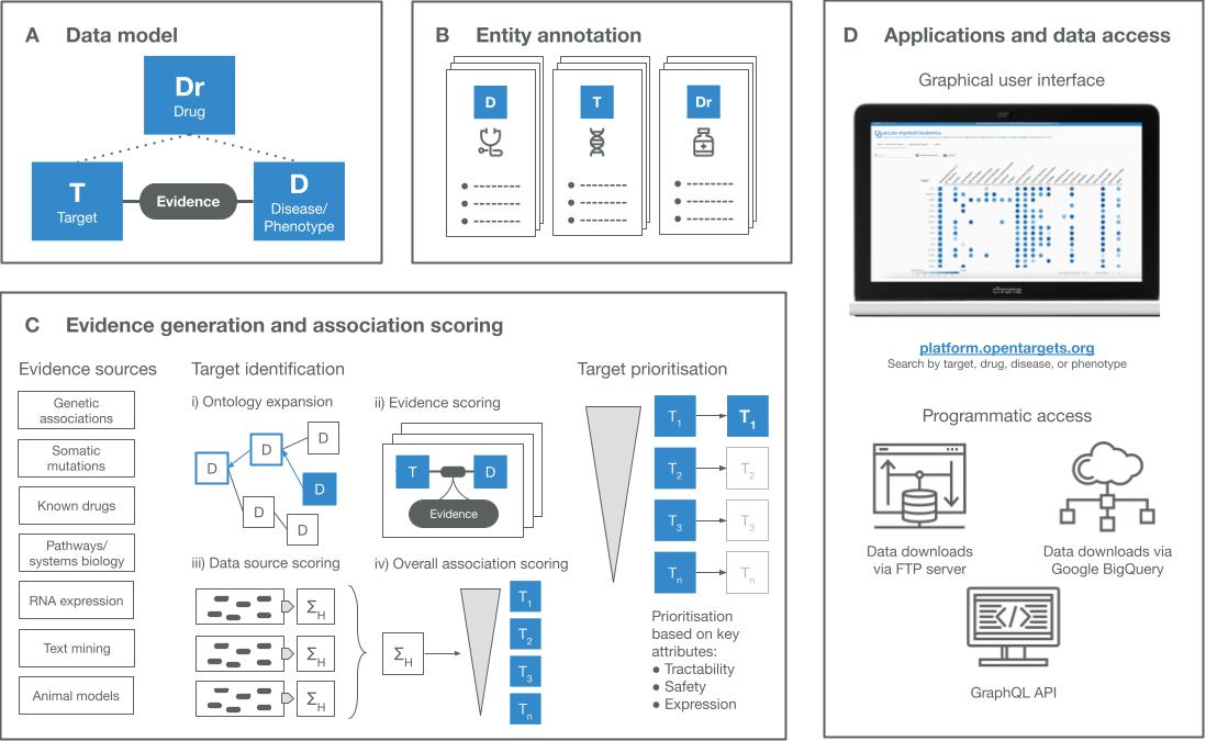
The English name of the disease, such as rheumatoid arthritis.
The type of data, including directly associated and all associated data.
The cutoff value for the disease-target association score. Only target information with a score greater than this cutoff will be output.
The type of target, default is all representing all target classes.
The output includes files related to the disease and its targets:
| File Name | Description |
|---|---|
| disease_info.csv | Disease information table |
| target_info.csv | Target information table |
| targets_by_data_source.csv | Disease-target association scores by data source |
| targets_by_data_type.csv | Disease-target association scores by data type |
| uniprot_ids.txt | List of target protein UniProt IDs |
| genes.txt | List of target gene names |
Structure Minimization是结构优化模块,支持氢原子优化、氨基酸侧链优化、整体优化三种方式。
结构文件,PDB格式。
优化类型,支持以下几种:
hydrogen:约束限制所有非氢原子,对结构上的氢原子进行优化。
sidechain:约束蛋白骨架,优化蛋白氨基酸侧脸,若存在小分子,整个小分子进行限制。
all:系统整体优化,不做任何限制约束。
可多选,进行多步优化。
能量优化的步数。
采用的分子力场,默认ff14SB。ff19SB, ff14SB适合蛋白和核酸的凝聚相模拟,也支持小分子。
约束力常数,单位为kcal/mol/Å^2,数值越大,约束能力越强。
输出文件名称,默认minimized_structure.pdb。
输出结果为优化后的结构文件minimized_structure.pdb,保留了输入文件中的链和氨基酸编号信息。
The Structure Minimization module is used for structural optimization, supporting three types of optimizations: hydrogen atom optimization, amino acid side chain optimization, and overall optimization.
The structure file in PDB format.
The type of optimization, supporting the following options:
The number of steps for energy optimization.
The molecular force field used, default is ff14SB. ff19SB and ff14SB are suitable for condensed phase simulations of proteins and nucleic acids, and also support small molecules.
The restrain force constant, in units of kcal/mol/Ų. The larger the value, the stronger the constraint.
The name of the output file, default is minimized_structure.pdb.
The output is the optimized structure file minimized_structure.pdb, retaining the chain and amino acid numbering information from the input file.
蛋白结构处理模块,用于补全缺失原子和残基,以及蛋白氨基酸残基的质子化判断以及加氢操作。采用pdbfixer补全缺失,采用propka3进行质子化判断。
蛋白的结构文件,PDB格式
提取指定链处理,默认all,代表选择全部链,输入链名,多条链用英文逗号隔开,如A,B表示从PDB文件中提取A,B链进行结构处理。注意链名之间不要用空格。
删除非标准蛋白或核酸残基,如水、离子、以及其他PDB中HETATM记录。
all:表示删除所有HETATM记录,包括水、离子、小分子等;
water:表示仅删除水;
ions:表示仅删除离子,默认为NA,CL;
custom:表示需要删除其他定制的残基名称,由Custom Heterogens参数指定。
Heterogens详细介绍可参考:https://www.wwpdb.org/documentation/file-format-content/format23/sect4.html
自定义Heterogens的残基名称,多个用英文逗号分隔,如ZN,MG
删除氢原子,Yes表示删除,No表示不删除。
添加缺失的重原子或者残基。
heavy:表示添加缺失重原子
residues:表示添加缺失残基,默认也会添加缺失的原子
是否进行质子化判断并添加氢原子,采用propka方法进行蛋白残基的质子化判断。
Yes:代表根据质子化判断结果进行加氢操作,
No:代表不加氢处理
用于蛋白质子化状态判断的pH值。
输出PDB文件中残基和原子的命名方式。
PDB:标准氨基酸格式,如组氨酸为HIS;
AMBER:AMBER格式,如组氨酸为HID/HIE/HIP;
CHARMM:CHARMM格式,如组氨酸为HSE/HSD/HSP。
输出的处理后的蛋白结构文件,PDB格式。默认文件名为:prepared_structure.pdb。
输出处理好的结构文件,PDB格式。文件中的原子和残基类型按照指定Naming Scheme方法。
The Structure Preparation module is used for completing missing atoms and residues in protein structures, as well as determining the protonation states of amino acid residues and adding hydrogen atoms. It uses pdbfixer for completing missing parts and propka3 for protonation state determination.
The protein structure file in PDB format.
Specify the chains to be processed. The default is all, which means all chains will be processed. To specify chains, input the chain names separated by commas without spaces, e.g., A,B to process chains A and B from the PDB file.
Remove non-standard protein or nucleic acid residues such as water, ions, and other HETATM records in the PDB.
NA,CL.Custom Heterogens parameter.For more details on Heterogens, refer to: Heterogen Information
Specify custom heterogens to be removed by their residue names, separated by commas, e.g., ZN,MG.
Remove hydrogen atoms.
Add missing heavy atoms or residues.
Determine protonation states and add hydrogen atoms using the propka method.
The pH value used for determining the protonation states of the protein residues.
The naming convention for residues and atoms in the output PDB file.
The name of the output processed protein structure file in PDB format. The default file name is prepared_structure.pdb.
The output is a processed structure file in PDB format. The atoms and residue types in the file follow the specified naming scheme.

Antibody RMSD模块对参考抗体结构及其他CDR相同的抗体结构,进行基于Fv区域的结构叠合,并计算CDR区域的RMSD值。支持普通抗体及纳米抗体。
应用场景:人源化后的抗体序列,预测抗体结构后,比较各结构CDR区域的RMSD差异。支持普通抗体及纳米抗体。
多个抗体结构PDB文件的压缩打包文件,TAR格式
进行RMSD计算的参考抗体结构,PDB格式
抗体叠合结构输出名称,TAR.GZ格式
result.csv ,包含信息如下:| 列名 | 说明 |
|---|---|
| Reference Antibody | 参考抗体结构的名称 |
| Target | 用于计算RMSD的其他抗体结构名称 |
| H.CDR1 | H链CD1R区域的RMSD值 |
| H.CDR2 | H链CDR2区域的RMSD值 |
| H.CDR3 | H链CDR3区域的RMSD值 |
| H.CDR | H链CDR区域整体的RMSD值 |
| L.CDR1 | L链CDR1区域的RMSD值 |
| L.CDR2 | L链CDR2区域的RMSD值 |
| L.CDR3 | L链CDR3区域的RMSD值 |
| L.CDR | L链CDR区域整体的RMSD值 |
| CDR_ALL | CDR区域整体的RMSD值 |
The Antibody RMSD module aligns the reference antibody structure with other antibodies having the same CDR regions, performs a structural overlay based on the Fv regions, and calculates the RMSD values of the CDR regions.
Application Scenario: After humanizing antibody sequences and predicting antibody structures, the module compares the RMSD differences in the CDR regions of various structures.
Compressed TAR file containing multiple antibody structure PDB files.
Reference antibody structure in PDB format for RMSD calculation.
Antibody composite structure output name, TAR.GZ format
result.csv, including the following information:| Column Name | Description |
|---|---|
| Reference Antibody | Name of the reference antibody structure |
| Target | Name of the other antibody structure used for RMSD calculation |
| H.CDR1 | RMSD value of the H-chain CDR1 region |
| H.CDR2 | RMSD value of the H-chain CDR2 region |
| H.CDR3 | RMSD value of the H-chain CDR3 region |
| H.CDR | Overall RMSD value of the H-chain CDR regions |
| L.CDR1 | RMSD value of the L-chain CDR1 region |
| L.CDR2 | RMSD value of the L-chain CDR2 region |
| L.CDR3 | RMSD value of the L-chain CDR3 region |
| L.CDR | Overall RMSD value of the L-chain CDR regions |
| CDR_ALL | Overall RMSD value of all CDR regions |
Target Prediction (FastTargetPred)是基于二维相似度的小分子靶点预测模块,活性分子及靶点数据来源于ChEMBL25数据库,相似度计算采用1024位ECFP4的分子指纹,特点是速度块,几小时完成数十万化合物的靶点预测。
小分子结构文件,SDF格式
相似度(Tanimoto)阈值。从ChEMBL中查找大于相似度阈值的化合物。
输出文件名称
输出结果包括:
| 输出文件名称 | 说明 |
|---|---|
| result.csv | 靶点预测结果的csv文件 |
| result.html | 靶点预测结果的html文件 |
其中输出结果包含信息如下:
| 字段名称 | 说明 |
|---|---|
| Query name | 查询分子名称 |
| Database molecule id | ChEMBL中相似找出的相似分子ID |
| Target id | 靶标分子ID |
| Score | 相似度数值 |
| Uniprot | 蛋白Uniprot ID |
| Uniprot name | Uniprot分子名称 |
| Status | 数据发表情况 |
| Protein names | 蛋白名称 |
| Gene names | 基因名称 |
| Organism | 物种名称 |
| CHEMBL | 靶点CHEMBL分子ID |
| Involvement in disease | 参与疾病类型 |
| Geneontology (biological process) | 谱系学(生物过程) |
| Cross-reference (Reactome) | 交叉引用(Reactome) |
Chaput L, Guillaume V, Singh N, Deprez B, Villoutreix BO. FastTargetPred: a program enabling the fast prediction of putative protein targets for input chemical databases. Bioinformatics. 2020 Aug 15;36(14):4225-4226.https://doi.org/10.1093/bioinformatics/btaa494
Target Prediction (FastTargetPred) is a module for predicting small molecule targets based on 2D similarity. The active molecules and target data are sourced from the ChEMBL25 database. Similarity calculation uses 1024-bit ECFP4 molecular fingerprints. The main feature of this module is its speed, capable of predicting targets for hundreds of thousands of compounds within a few hours.
The structure file of small molecules in SDF format.
The similarity (Tanimoto) threshold. Compounds from ChEMBL with a similarity greater than this threshold will be considered.
The name of the output file.
The output results include:
| Output File Name | Description |
|---|---|
| result.csv | CSV file containing the target prediction results |
| result.html | HTML file containing the target prediction results |
The output results contain the following information:
| Field Name | Description |
|---|---|
| Query name | Name of the query molecule |
| Database molecule id | ID of the similar molecule found in ChEMBL |
| Target id | ID of the target molecule |
| Score | Similarity score |
| Uniprot | Uniprot ID of the protein |
| Uniprot name | Name of the Uniprot molecule |
| Status | Publication status of the data |
| Protein names | Names of the proteins |
| Gene names | Names of the genes |
| Organism | Name of the organism |
| CHEMBL | CHEMBL molecule ID of the target |
| Involvement in disease | Types of diseases involved |
| Geneontology (biological process) | Gene ontology (biological process) |
| Cross-reference (Reactome) | Cross-reference (Reactome) |
静电势(ESP,electrostatic potential)表面是指在分子周围某个曲面上静电势的分布,通过静电势对蛋白质表面着色有助于识别带电分子或极性分子的结合位点。正电位区域与负电荷互补,而负电位区域与正电荷互补。蛋白质静电势对于蛋白质的稳定性、折叠、酶催化、蛋白质间相互作用以及与其他分子的结合等方面起着关键作用。APBS(Adaptive Poisson-Boltzmann Solver )是业界著名的计算生物大分子结构静电势能的工具。
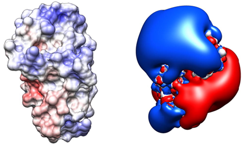
蛋白结构文件,PDB格式
输出文件格式,支持DX或者CUBE
输出静电势能结果文件potential.dx或者potential.cube,用于将静电势能渲染到蛋白表面上。
Electrostatic potential (ESP) surfaces represent the distribution of electrostatic potential around a molecule on a given surface. Coloring the protein surface based on electrostatic potential helps identify binding sites for charged or polar molecules. Regions with positive potential complement negatively charged molecules, while regions with negative potential complement positively charged molecules. Protein electrostatic potential plays a crucial role in protein stability, folding, enzymatic catalysis, protein-protein interactions, and binding with other molecules. APBS (Adaptive Poisson-Boltzmann Solver) is a renowned tool for calculating the electrostatic potential of biological macromolecules.
The protein structure file in PDB format.
The format of the output file, supporting DX or CUBE.
The output electrostatic potential result file, named potential.dx or potential.cube, can be used to render the electrostatic potential on the protein surface.
通过蛋白序列逆折叠模型ESM-IF,预测蛋白质的绝对稳定性ΔG。
传统的物理方法(如FoldX、Rosetta等)预测蛋白稳定性ΔG,依赖于高置信度结构pdb,如果突变太多,结构置信度降低,预测结果较差。在ProteinGym的benchmark结果表明,生成模型ESM-IF在zero-shot预测DMS数据的蛋白突变稳定性ΔΔG达到同类最佳水平。该方法是在突变预测基础上的延伸,利用ESM-IF模型直接预测完整蛋白折叠稳定性的绝对ΔG值。
经过测试,预测误差RMSE ≈ 1.5 kcal/mol,相关系数为0.7,是预测蛋白质的折叠稳定性ΔG的重大突破。
原理:
然后,将蛋白质所有氨基酸位点的Lk加和,得到蛋白整体的log-likelihood。
最后,通过线性整体log-likelihood与实验稳定性ΔG拟合得到拟合参数,根据a/b就可以将log-likelihood转换成蛋白稳定性ΔG了。
模型预测效果如下图所示:
在两个不同数据集的 265 种蛋白质的预测稳定性值和实验稳定性值进行了比较。Spearman相关系数 (ρs) 为0.69,误差RMSE约为1.36 kcal/mol,相关性较好。
与其他基线模型比较结果如下图所示:
蛋白结构文件,PDB格式
多个蛋白结构PDB的压缩文件,支持格式:.zip、.tar、.tar.gz、.tgz、.tar.bz2、.tbz2、.tar.xz、.txz
当同时上传蛋白结构PDB和压缩包时会合并计算。
| 列名 | 说明 |
|---|---|
| Name | 结构名称 |
| Absolute_Folding_Stability (kcal/mol) | dG,越大越好,代表去折叠状态能量减去折叠状态能量,即去折叠需要的能量值,通常为正值,能量越大表示需要能量越多,折叠状态越稳定 |
Predicting absolute protein folding stability using generative models Matteo Cagiada, Sergey Ovchinnikov, Kresten Lindorff-Larsen bioRxiv 2024.03.14.584940; https://doi.org/10.1101/2024.03.14.584940
The absolute folding stability ($\Delta G$) of a protein can be predicted using the inverse folding model ESM-IF. Traditional physical methods (such as FoldX, Rosetta, etc.) for predicting protein stability $\Delta G$ rely on high-confidence structure PDB files. If mutations are numerous, the structural confidence decreases, leading to poor prediction results. Benchmark results from ProteinGym show that the generative model ESM-IF achieves state-of-the-art performance in zero-shot prediction of protein mutation stability $\Delta \Delta G$ on DMS data. This method extends mutation prediction by using the ESM-IF model to directly predict the absolute $\Delta G$ value of the complete protein folding stability.
Testing shows a prediction error RMSE of approximately 1.5 kcal/mol and a correlation coefficient of 0.7, marking a significant breakthrough in predicting the folding stability $\Delta G$ of proteins.
Principle
The log-likelihood of the entire protein is obtained by summing the $L_k$ values of all amino acid sites. Finally, the log-likelihood is linearly fitted to the experimental stability $\Delta G$ to obtain the fitting parameters. The log-likelihood can be converted into protein stability $\Delta G$ based on $a/b$.
Model Prediction Performance
The predicted stability values and experimental stability values for 265 proteins in two different datasets were compared. The Spearman correlation coefficient ($\rho_s$) is 0.69, and the error RMSE is about 1.36 kcal/mol, indicating good correlation.
Comparison with Other Baseline Models
The protein structure file in PDB format.
Compressed archive file containing multiple protein structure PDBs. Supported formats: .zip, .tar, .tar.gz, .tgz, .tar.bz2, .tbz2, .tar.xz, .txz.and the compressed file are uploaded, they will be calculated together.
| Column Name | Description |
|---|---|
| Name | Structure name |
| Absolute_Folding_Stability (kcal/mol) | Delta G, the higher the better, representing the energy difference between the unfolded and folded states. It is usually a positive value, with higher values indicating greater stability in the folded state. |
De novo Generation (REINVENT4)是基于阿斯利康开源的REINVENT4算法用于小分子全新生成的模块。支持多种分子生成方式:Reinvent - 从头开始创造新类药分子,Libinvent - 修饰一个骨架,Linkinvent - 设计两个片段之间的linker,Mol2Mol - 在用户定义的相似度范围内优化分子。

从头生成新分子
生成的分子个数
输出CSV文件名称
输出SDF文件名称
对已有骨架结构进行修饰,生成含有该骨架结构的新分子。
小分子的骨架结构文件,该模式需要输入带 * 的小分子,SMILES或SDF格式,可以通过内嵌的wedraw工具来获得。
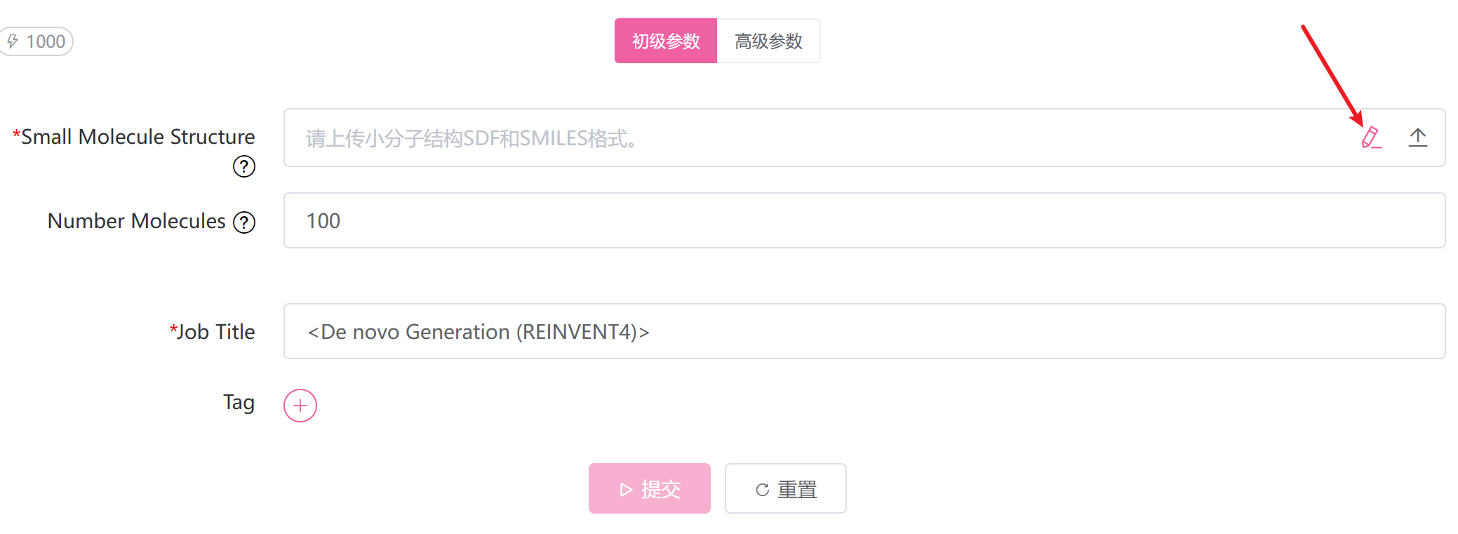
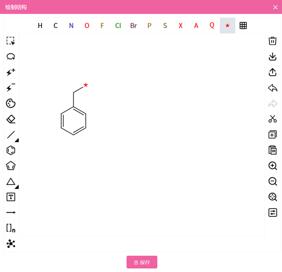
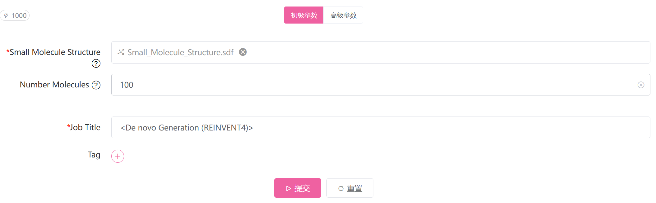
生成的分子个数。程序会按照该大小进行采样,随后自动过滤掉不符合设定片段拼接规则或子结构匹配要求的结果。因此,最终输出的有效样本数可能少于设定值。
输出CSV文件名称
输出SDF文件名称
对两个结构片段进行连接,生成linker结构,获得新分子。
小分子的骨架结构文件,该模式需要输入带 * 的两个小分子,SMILES或SDF格式,可以通过内嵌的wedraw工具来获得(同LibInvent模式)。
生成的分子个数。程序会按照该大小进行采样,随后自动过滤掉不符合设定片段拼接规则或子结构匹配要求的结果。因此,最终输出的有效样本数可能少于设定值。
输出CSV文件名称
输出SDF文件名称
优化分子结构,在用户定义的相似度范围内优化分子。
小分子的骨架结构文件,SMILES或SDF格式,可以通过内嵌的wedraw工具来获得。
生成的分子个数,程序会按照该大小进行采样,随后自动过滤掉不符合设定片段拼接规则或子结构匹配要求的结果。因此,最终输出的有效样本数可能少于设定值。注意:它乘以输入分子的个数为最终输出总分子数。
有5种不同的优化策略:
beamsearch或者multinomial
多项抽样中的温度
输出CSV文件名称
输出SDF文件名称
输出结果包括:
| 输出文件名称 | 说明 |
|---|---|
| result.csv | 全新生成的化合物CSV文件,包含了SMILES信息 |
| denovo.sdf | 全新生成的化合物SDF文件 |
De novo Generation (REINVENT4) is a module based on AstraZeneca’s open-source REINVENT4 algorithm for generating new small molecules. It supports various molecule generation methods: Reinvent - creating new drug-like molecules from scratch, Libinvent - modifying a scaffold, Linkinvent - designing a linker between two fragments, and Mol2Mol - optimizing molecules within a user-defined similarity range.
De novo generation of new molecules.
Number of molecules to generate.
Name of the output CSV file.
Name of the output SDF file.
Modify an existing scaffold to generate new molecules containing that scaffold.
The scaffold structure file of the small molecule. This mode requires a small molecule with * placeholders. Supported formats: SMILES or SDF. The embedded wedraw tool can be used to create such molecules.
Number of molecules to generate. The program will sample according to this value and then automatically filter out results that do not satisfy the defined fragment assembly rules or substructure matching requirements. Therefore, the final number of valid output samples may be smaller than the set value.
Name of the output CSV file.
Name of the output SDF file.
Connect two structural fragments to form a linker structure and generate new molecules.
The scaffold structure files of the two small molecules. This mode requires two small molecules with * placeholders. Supported formats: SMILES or SDF. The embedded wedraw tool can be used to create such molecules (same as in LibInvent mode).
Number of molecules to generate. The program will sample according to this value and then automatically filter out results that do not satisfy the defined fragment assembly rules or substructure matching requirements. Therefore, the final number of valid output samples may be smaller than the set value.
Name of the output CSV file.
Name of the output SDF file.
Optimize molecular structures within a user-defined similarity range.
The scaffold structure file of the small molecule. Supported formats: SMILES or SDF. The embedded wedraw tool can be used to create such molecules.
Number of molecules to generate. The program will sample according to this value and then automatically filter out results that do not satisfy the defined fragment assembly rules or substructure matching requirements. Therefore, the final number of valid output samples may be smaller than the set value. Note: the final total number of output molecules is equal to this value multiplied by the number of input molecules.
There are five different optimization strategies:
beamsearch or multinomial
Temperature for multinomial sampling.
Name of the output CSV file.
Name of the output SDF file.
The output includes:
| Output File Name | Description |
|---|---|
| result.csv | CSV file containing newly generated compounds, including SMILES information |
| denovo.sdf | SDF file containing newly generated compounds |
该模块基于物理模型(分子力学经验力场)计算多个蛋白结构的能量,并与参考蛋白结构的能量进行比较。
多个蛋白结构PDB文件的压缩打包文件,TAR格式
进行能量比对的参考蛋白结构,PDB格式
| 列名 | 说明 |
|---|---|
| Name | 结构名称 |
| Score | 能量打分,数值负得越多表示能量越低 |
This module calculates the energy of multiple protein structures based on a physical model (empirical molecular force field) and compares these energies with the energy of a reference structure.
Compressed TAR file containing multiple protein structure PDB files.
Reference structure in PDB format for energy comparisons.
| Column Name | Description |
|---|---|
| Name | Structure name |
| Score | Energy score, where a more negative value indicates lower energy |
该模块基于ESM大规模预训练蛋白语言模型实现。提取序列的向量化特征信息(embeddings),可用于下游序列性质(如:突变对应的亲和力变化、稳定性变化,抗体序列可开发性等)预测任务,为判别模型的训练提供序列特征。
ESM模型是通用蛋白质语言模型,采用UniRef50/90等序列数据库(数千万条序列)进行模型训练,提供了不同参数量(800万,3500万,1.5亿,6.5亿,30亿,150亿)的各类模型,可用于直接从蛋白序列预测结构、功能和其他蛋白质性质。如在结构预测中,ESM避免了对外部进化数据库、MSA和模板的需求,计算精度与AlphaFold2(存在MSA信息时)接近,无可用MSA信息时,计算精度ESM要显著优于AlphaFold2。计算速度比AlphaFold2快数十倍。
蛋白的序列文件,FASTA格式
注意:多条序列时,序列名称应避免重复,模块会对重复的序列名称进行重命名,格式为“原序列名_数字”
选择用于提取序列特征的模型,可用模型及特征维度说明如下:
| 模型名称 | 参数量 | 特征维度 | 模型层数 |
|---|---|---|---|
| ESM1b_650M | 650M | 1280 | 33 |
| ESM1v_650M | 650M | 1280 | 33 |
| ESM2_8M | 8M | 320 | 6 |
| ESM2_35M | 35M | 480 | 12 |
| ESM2_150M | 150M | 640 | 30 |
| ESM2_650M | 650M | 1280 | 33 |
| ESM2_3B | 3B | 2560 | 36 |
| ESM2_15B | 15B | 5120 | 48 |
备注:“M”表示Million(百万),“B”表示Billion(十亿),ESM-2-15B模型需要的GPU卡显存大小约为32GB
每条序列会输出一个特征信息文件“序列名.pt”,包含了该序列的向量化特征信息,该特征信息由模型最后一层产生。多条序列会输出多个pt文件,并压缩为feats.tar压缩文件。
特征信息文件可通过torch加载,如下:
embs = torch.load(“序列名.pt”)
embs[‘mean_representations’][‘模型层数’]
This module is based on the ESM (Evolutionary Scale Modeling) large-scale pre-trained protein language model. It extracts vectorized feature information (embeddings) from sequences, which can be used for downstream sequence property prediction tasks such as changes in affinity and stability corresponding to mutations, developability of antibody sequences, etc., providing sequence features for discriminative model training.
The ESM model is a universal protein language model trained on sequence databases such as UniRef50/90 (tens of millions of sequences). It offers various models with different parameter sizes (8 million, 35 million, 150 million, 650 million, 3 billion, 15 billion) that can be used to predict protein structures, functions, and other protein properties directly from protein sequences. In structural prediction, ESM eliminates the need for external evolutionary databases, multiple sequence alignments (MSA), and templates. Its calculation accuracy is comparable to AlphaFold2 (when MSA information is available) and significantly superior to AlphaFold2 in accuracy when MSA information is not available. ESM is also several times faster than AlphaFold2.
The sequence file of the protein in FASTA format.
Note: When multiple sequences are provided, sequence names should be unique to avoid duplication. The module will rename duplicated sequence names in the format “original_sequence_name_number”.
Select the model used to extract sequence features. The available models and their feature dimensions are as follows:
| Model Name | Parameters | Feature Dimension | Number of Layers |
|---|---|---|---|
| ESM1b_650M | 650M | 1280 | 33 |
| ESM1v_650M | 650M | 1280 | 33 |
| ESM2_8M | 8M | 320 | 6 |
| ESM2_35M | 35M | 480 | 12 |
| ESM2_150M | 150M | 640 | 30 |
| ESM2_650M | 650M | 1280 | 33 |
| ESM2_3B | 3B | 2560 | 36 |
| ESM2_15B | 15B | 5120 | 48 |
Note: “M” stands for Million, “B” stands for Billion. The ESM-2-15B model requires approximately 32GB of GPU memory.
Each sequence will output a feature information file named “sequence_name.pt,” which contains the vectorized feature information of that sequence generated by the last layer of the model. For multiple sequences, multiple pt files will be output and compressed into a feats.tar file.
The feature information file can be loaded using torch as follows:
embs = torch.load(“sequence_name.pt”)
embs[‘mean_representations’][‘number_of_layers’]
该模块用于NGS测序后的DNA序列(抗体)分析,具体分析内容包括:
NGS测序后的DNA序列,FASTA/AB1格式
注意:当前限制输入序列为1000条。
物种类型,支持2种:HUMAN, MOUSE。默认为HUMAN
编号规则,支持imgt, chothia, kabat
氨基酸序列聚类方案,支持2种:full, cdr。‘full’表示使用全长序列进行聚类,‘cdr’表示使用CDR序列进行聚类(具体CDR位置在参数‘CDRs’中设定),默认为‘cdr’
指定用于聚类的CDR区域,在‘Cluster’参数为cdr时生效。可选区域为(支持多选):CDR1,CDR2,CDR3。默认选择CDR3。
聚类中采用的序列一致性数值,范围在0-1之间,默认值为0.5
聚类前是否要求IGV基因名称一致的序列归为一组,默认为False
输出结果文件名,默认为NGS_res.csv
NGS测序后的蛋白序列,FASTA格式
注意:当前限制输入序列为1000条。
物种类型,支持2种:HUMAN, MOUSE。默认为HUMAN
编号规则,支持imgt, chothia, kabat
氨基酸序列聚类方案,支持2种:full, cdr。‘full’表示使用全长序列进行聚类,‘cdr’表示使用CDR序列进行聚类(具体CDR位置在参数‘CDRs’中设定),默认为‘cdr’
指定用于聚类的CDR区域,在‘Cluster’参数为cdr时生效。可选区域为(支持多选):CDR1,CDR2,CDR3。默认选择CDR3。
聚类中采用的序列一致性数值,范围在0-1之间,默认值为0.5
聚类前是否要求IGV基因名称一致的序列归为一组,默认为False
输出结果文件名,默认为NGS_res.csv
输出result.csv结果文件,包含以下信息:
| 列名 | 说明 | 备注 |
|---|---|---|
| ID | 序列名称 | |
| DNA_Seq | DNA序列 | |
| Protein_Seq | 翻译后的氨基酸序列 | |
| Chain | 链类型:IGH/IGK/IGL | |
| CDR1_AA | CDR1的氨基酸序列 | |
| CDR2_AA | CDR2的氨基酸序列 | |
| CDR3_AA | CDR3的氨基酸序列 | |
| CDR1_Length | CDR1的氨基酸序列长度 | |
| CDR2_Length | CDR2的氨基酸序列长度 | |
| CDR3_Length | CDR3的氨基酸序列长度 | |
| Unusual_Residue(ESM) | 基于ESM模型的不常见残基及优势突变 | 如:'V11L’表示序列中第11位的V是模型判定的该位置不常见残基,L为模型判定的该位置优势突变残基 |
| Unusual_Residue(IgLM) | 基于IgLM模型的不常见残基及优势突变 | 同上 |
| V_Gene_First | 匹配的首个IGV基因名称。 | IGV基因名称可能存在多个匹配,这里列出首个。注:输入为蛋白序列时,该字段忽略。 |
| V_Gene | IGV基因名称 | 如同时匹配多个基因名,用‘;’分隔 |
| D_Gene | IGD基因名称 | 同上,注:输入为蛋白序列时,该字段忽略。 |
| J_Gene | IGJ基因名称 | 同上,注:输入为蛋白序列时,该字段忽略。 |
| CDR1_Highrisk_Hotspots | CDR1中的PTM高风险位点 | 如:‘NG(1)’表示高风险位点‘NG’出现1次 |
| CDR2_Highrisk_Hotspots | CDR2中的PTM高风险位点 | 同上 |
| CDR3_Highrisk_Hotspots | CDR3中的PTM高风险位点 | 同上 |
| CDR1_Lowrisk_Hotspots | CDR1中的PTM低风险位点 | 同上 |
| CDR2_Lowrisk_Hotspots | CDR2中的PTM低风险位点 | 同上 |
| CDR3_Lowrisk_Hotspots | CDR3中的PTM低风险位点 | 同上 |
| Mutations(AA) | 与Germline序列比对所对应的突变,并标注了突变所在区域(FR或CDR),多个突变用分号分隔 | 如: 'V29I(CDR1)'表示编号29的残基存在突变,其中Germline序列中残基是V,当前抗体序列中残基为I,根据抗体编号规则所在的区域为CDR1 |
| SHM(AA) | 基于氨基酸序列计算得到的体系超突变率 | SHM: Somatic hypermutation,计算方式是将当前序列与Germline参考序列进行比对,序列突变总数量与序列长度的比值即为SHM |
| SHM(NA) | 基于DNA序列计算得到的体系超突变率 | 同上,注:输入为蛋白序列时,该字段忽略。 |
| pI | 等电点 | |
| kDa | 分子量(千道尔顿) | |
| Hydrophobicity | 疏水性指数 | 序列各氨基酸的Kyte-Doolittle疏水指数之和,主要用来快速粗略比较近似序列的相对疏水程度高低 |
| Pre_Cluster_Group | 聚类分析中的组别名称 | 序列聚类前先进行序列分组,各组内序列再进行聚类分析。当选择CDR聚类时,CDR序列长度一致的序列归为一组。组别名称由各聚类参数组合而成,如:组名为‘8_8_18’,表示该组由CDR1,2,3长度分别为8,8,18的多条序列组成。如果分组参数设定要求IGV基因名称一致,则IGV基因名称也会出现在组别名称中,如:‘8_8_18_IGKV1-12*01’ |
| Cluster_ID | 序列所属类别的名称 | 如:‘2_3’表示第2组第3个类别 |
| Cluster_Size | 序列所属类别包含的序列数目 | 如:‘5’表示该类别含有5条序列 |
| Cluster_Center | 序列是否为聚类中心 | '1’表示是,‘0’表示不是 |
| Cluster_Ident | 聚类后的类别中,成员序列与聚类中心序列的序列一致性 | 聚类时,如果选择全长序列聚类,这里即为全长序列的一致性;如选择CDR进行聚类,则为选中的CDR区域序列的整体一致性 |
| Cluster_CDR1_Ident | 聚类后的类别中,成员序列与聚类中心序列的CDR1序列的一致性 | |
| Cluster_CDR2_Ident | 聚类后的类别中,成员序列与聚类中心序列的CDR2序列的一致性 | |
| Cluster_CDR3_Ident | 聚类后的类别中,成员序列与聚类中心序列的CDR3序列的一致性 | |
| Unique_ID | 唯一序列编号 | 从 1 开始按出现顺序递增,表示该序列所属的唯一序列簇。若 CDR3 区域差异 ≥ 1 个残基,则判定为不同序列;或 CDR1 + CDR2 + CDR3 区域的总差异 ≥ 3 个残基,也判定为不同序列;若上述条件均不满足,则判定为相同序列。 |
| Dup_Count | Unique_ID 对应的序列在原始数据中出现的重复次数 |
输出进化树信息,为打包文件tree.tar,包含多个进化树文件tree_clusterXXX.txt,每个进化树文件包含该聚类类别(cluster)中所有成员序列CDR区域的进化分析结果。
风险位点说明:

其中打勾标记的位点NXS, NXT, NG, DHK, DG, DD和Cys共7个位点为默认的潜在PTM高风险位点,通常需重点关注,其余为低风险位点。
The module is used for the analysis of the DNA sequence (antibody) after NGS sequencing. The analysis content includes:
-IGV, IGD, IGJ gene annotation(IGBLAST)
-DNA sequence is translated as amino acid sequence (antibody) and CDR recognition
-Based on protein (antibody) language model, analyze unusual residual and advantageous mutations (ESM, IgLM)
-PTM (post -translation modification) hotspot analysis, low and high risk hotspot
-Sequence property calculation (PI, molecular weight, hydrophobicity)
-Sequence clustering(MMSEQ2)
DNA sequence after NGS sequencing,FASTA/ab1 format
Note : The current entry limit is 1000 entries.
Type of Species,support two:HUMAN, MOUSE. The default is HUMAN
Numbering scheme: imgt, chothia and kabat
Scheme of sequence clustering,support two:full, cdr. ‘full’ means clustering by full length sequence,‘cdr’ means clustering by CDR. The default is ‘cdr’
Specify the CDRs for clustering,when the ‘Cluster’ is set to ‘cdr’. Mutiple choice are supported: CDR1, CDR2, CDR3
The sequence identity used for clustering,value range from 0 to 1, the default is 0.5
Whether the sequence of the IGV gene name is consistent for classification as a group before clustering. The default is False
Result file, default is NGS_res.csv
Protein sequence after NGS sequencing,FASTA format
Note : The current entry limit is 1000 entries.
Type of Species,support two:HUMAN, MOUSE. The default is HUMAN
Numbering scheme: imgt, chothia and kabat
Scheme of sequence clustering,support two:full, cdr. ‘full’ means clustering by full length sequence,‘cdr’ means clustering by CDR. The default is ‘cdr’
Specify the CDRs for clustering,when the ‘Cluster’ is set to ‘cdr’. Mutiple choice are supported: CDR1, CDR2, CDR3
The sequence identity used for clustering,value range from 0 to 1, the default is 0.5
Whether the sequence of the IGV gene name is consistent for classification as a group before clustering. The default is False
Result file, default is NGS_res.csv
Export the result file result.csv, which includes the following information:
| Field Name | Description | Notes |
|---|---|---|
| ID | Sequence | name |
| DNA_Seq | DNA sequence | |
| Protein_Seq | Translated amino acid sequence | |
| Chain | Chain type: IGH/IGK/IGL | |
| CDR1_AA | Amino acid sequence of CDR1 | |
| CDR2_AA | Amino acid sequence of CDR2 | |
| CDR3_AA | Amino acid sequence of CDR3 | |
| CDR1_Length | Length of CDR1 amino acid sequence | |
| CDR2_Length | Length of CDR2 amino acid sequence | |
| CDR3_Length | Length of CDR3 amino acid sequence | |
| Unusual_Residue(ESM) | Uncommon residues and dominant mutations based on the ESM model | e.g., ‘V11L’ indicates that the V at position 11 in the sequence is determined by the model to be an uncommon residue, and L is determined by the model to be a dominant mutation residue at that position |
| Unusual_Residue(IgLM) | Uncommon residues and dominant mutations based on the IgLM model | Same as above |
| V_Gene_First | The name of the first IGV gene that matches. | There may be multiple matches for IGV gene names, the first of which is listed here |
| V_Gene | Name of the IGV gene | If multiple gene names match simultaneously, separate them with ‘;’ |
| D_Gene | Name of the IGD gene | Same as above |
| J_Gene | Name of the IGJ gene | Same as above |
| CDR1_highrisk_hotspots | PTM high-risk sites in CDR1 | e.g., ‘NG(1)’ indicates the high-risk site ‘NG’ appears 1 time |
| CDR2_Highrisk_hotspots | PTM high-risk sites in CDR2 | Same as above |
| CDR3_Highrisk_hotspots | PTM high-risk sites in CDR3 | Same as above |
| CDR1_Lowrisk_hotspots | PTM low-risk sites in CDR1 | Same as above |
| CDR2_Lowrisk_hotspots | PTM low-risk sites in CDR2 | Same as above |
| CDR3_Lowrisk_hotspots | PTM low-risk sites in CDR3 | Same as above |
| Mutations(AA) | corresponds to mutations compared to the Germline sequence and annotates the region where the mutation occurs (FR or CDR), with multiple mutations separated by semicolons. For example, ‘V29I(CDR1)’ indicates a mutation at residue 29, where the residue in the Germline sequence is V and the residue in the current antibody sequence is I, and based on the antibody numbering rules, the region is identified as CDR1. | |
| SHM(AA) | System hypermutation rate calculated based on amino acid sequence | SHM: Somatic hypermutation is calculated by aligning the current sequence with a Germline reference sequence. The ratio of the total number of sequence mutations to the sequence length is defined as SHM |
| SHM(NA) | System hypermutation rate calculated based on DNA sequence | Same as above |
| pI | Isoelectric point | |
| kDa | Molecular weight (kilodalton) | |
| Hydrophobicity | Hydrophobicity index | The sum of the Kyte-Doolittle hydrophobicity indices of each amino acid in the sequence, mainly used for a rough comparison of the relative hydrophobicity levels of approximate sequences |
| Pre_Cluster_Group | Group name in cluster analysis | Before sequence clustering, sequences are grouped, and sequences within each group are then analyzed for clustering. For example, when selecting CDR clustering, sequences with the same CDR length are grouped together. The group name is composed of various clustering parameters, e.g., ‘8_8_18’ indicates that the group consists of multiple sequences with CDR1, 2, 3 lengths of 8, 8, 18, respectively |
| Cluster_ID | Name of the category to which the sequence belongs | e.g., ‘2_3’ indicates the third category in the second group |
| Cluster_Size | Number of sequences contained in the category | e.g., ‘5’ indicates that this category contains 5 sequences |
| Cluster_Center | Whether the sequence is a cluster center | ‘1’ indicates yes, ‘0’ indicates no |
| Cluster_Ident | Consistency of member sequences with the cluster center sequence in the clustered category | During clustering, if full-length sequence clustering is selected, this represents the consistency of the full-length sequences; if CDR clustering is chosen, it represents the overall consistency of the selected CDR region sequences |
| Cluster_CDR1_Ident | Consistency of member sequences with the CDR1 sequence of the cluster center sequence in the clustered category | |
| Cluster_CDR2_Ident | Consistency of member sequences with the CDR2 sequence of the cluster center sequence in the clustered category | |
| Cluster_CDR3_Ident | Consistency of member sequences with the CDR3 sequence of the cluster center sequence in the clustered category | |
| Unique_ID | Unique sequence ID | A unique sequence identifier, starting from 1 and incremented in order of appearance, representing the cluster to which the sequence belongs. Sequences are considered different if the CDR3 region differs by ≥ 1 residue, or if the total number of differences across CDR1 + CDR2 + CDR3 is ≥ 3 residues. If neither condition is met, sequences are considered identical. |
| Dup_Count | The number of times the sequence associated with the same Unique_ID appears in the original dataset. |
Output evolutionary tree information into a packed file named tree.tar, which includes multiple evolutionary tree files named tree_clusterXXX.txt, with each evolutionary tree file containing the evolutionary analysis results of the CDR regions of all member sequences in that clustering category (cluster).
Risk Site Description:
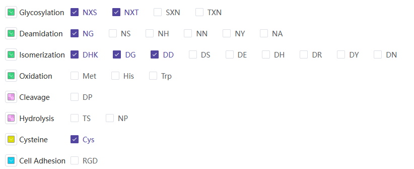
The default potential PTM high-risk sites marked with check marks include NXS, NXT, NG, DHK, DG, DD, and Cys, totaling 7 sites. These sites typically require special attention, while the rest are considered low-risk sites.
基于输入的9肽片段, 在人源片段库中搜索最相似的9肽片段。
人源片段库来源:
九肽片段,多个肽段用逗号分隔,例如:
NFFWHLHFP,GKGITLSVR,TPEALFVMT,GGIPIINCA,CVAIAEDRK
相同氨基酸的最小数量(相同位置),默认为7。
输出文件名称
输出结果文件为result.csv,包含信息如下:
| 字段名称 | 说明 |
|---|---|
| Query | 原始9肽 |
| Identity | 9肽中相同(保守)氨基酸的数目,越大越好,例如8代表有1个突变 |
| Target | 匹配到的9肽 |
| DiffMask | 以*号标记氨基酸差异的位置 |
| From | 生成片段的来源数据库 |
The Human Fragment BLAST is based on inputs of 9 peptides, searching the Germline, TCR, NextProt, OAS for the most similar 9 peptides.
The output file is result.csv and contains the following information:
| Field Name | Description |
|---|---|
| Query | original 9-mer peptide |
| Identity | The number of identical amino acids in the retrieved 9-mer peptide fragment. Greater value stands for less mutations. |
| Target | The resulting 9-mer peptides |
| DiffMask | The different positions of amino acids are marked with *. |
| From | The source database from which the fragment is generated. |
该模块基于RaptorX-Single算法实现,RaptorX-Single是一种基于单一序列的蛋白质结构预测方法,无需multiple sequence alignment(MSA)信息。它集成了多个蛋白质语言模型和一个结构生成模块,研究结果表明,RaptorX-Single除了比AlphaFold2等基于MSA的方法运行得更快之外,在预测抗体结构、极少同源序列的蛋白和单突变效应方面也优于AlphaFold2和其他无MSA的方法。当预测的蛋白序列有大量同源序列时,RaptorX-Single的预测结果也优于AlphaFold2。
RaptorX-Single的神经网络架构:
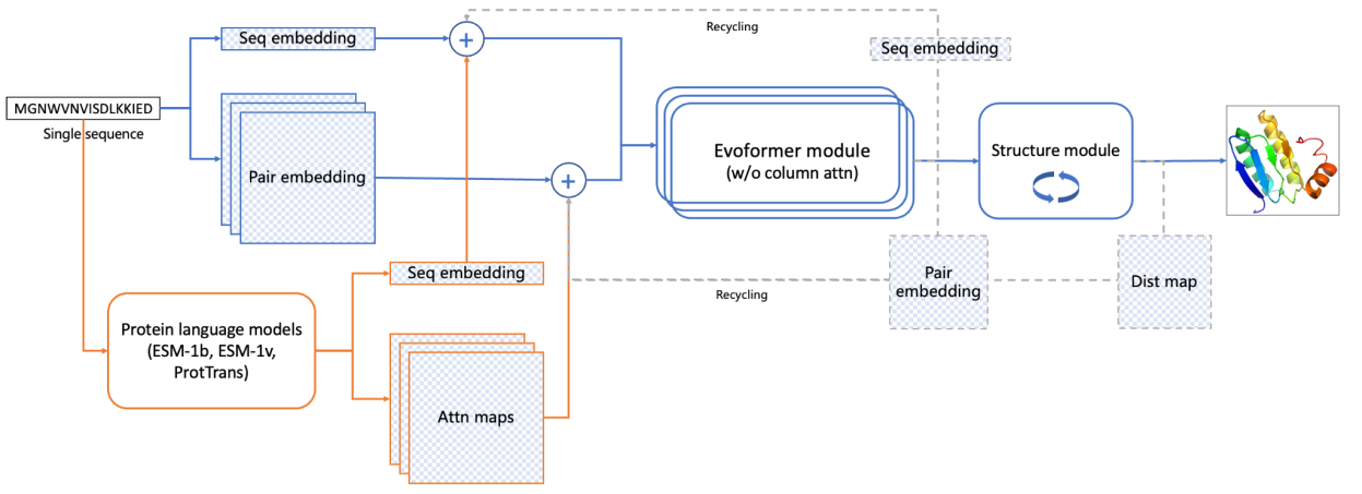
对抗体结构预测精度比较:

普通蛋白或抗体序列文件(不超过1000个氨基酸),FASTA格式,如:
>Nb21
MAQVQLVESGGGLVQAGGSLRLSCAVSGLGAHRVGWFRRAPGKEREFVAAIGANGGNTNYLDSVKGRFTISRDNAKNTIYLQMNSLKPQDTAVYYCAARDIETAEYTYWGQGTQVTVS
只支持预测单链蛋白或抗体,如果FASTA文件有多条链,每条链会单独预测为一个PDB结构。
选择预测结构时使用的模型,有两个模型可供选择:
protein表示蛋白模型,对应RaptorX-Single-ESM1b-ESM1v-ProtTrans.pt;
antibody表示抗体模型,对应RaptorX-Single-ESM1b-ESM1v-ProtTrans-Ab.pt。
如果预测蛋白,请选择前者,如果预测抗体,请选择后者
输出结果包括:
| 输出文件名称 | 说明 |
|---|---|
| first.pdb | 默认输出第一条序列的预测结构。 |
| structs.tar | 针对含有多条序列的fasta文件,压缩包中含所有的序列的预测结构。 |
RaptorX-Single: exploring the advantage of single sequence based protein structure prediction. Xiaoyang Jing, Fandi Wu, Jinbo Xu. bioRxiv 2023.04.24.538081
https://doi.org/10.1101/2023.04.24.538081
The module is implemented based on the RaptorX-Single algorithm, which is a single sequence-based protein structure prediction method that does not require multiple sequence alignment (MSA) information. It integrates multiple protein language models and a structure generation module. The results show that RaptorX-Single, in addition to running faster than MSA-based methods such as AlphaFold2, also outperforms AlphaFold2 and other MSA-free methods in predicting antibody structures, proteins with very few homologous sequences, and single mutation effects. RaptorX-Single also outperforms AlphaFold2 when predicting protein sequences with a large number of homologous sequences.
Network Architecture for RaptorX-Single:

Comparison of the accuracy of antibody structure prediction:
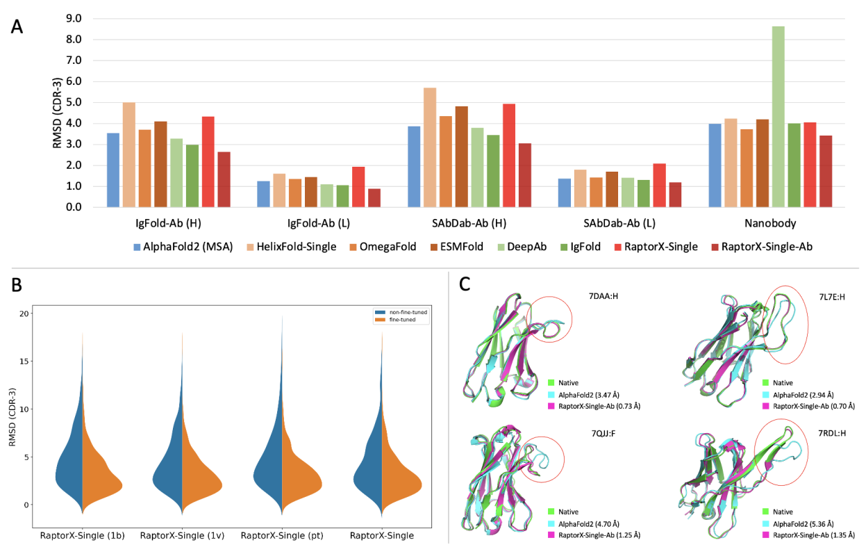
Protein or antibody sequence file (not more than 1000 amino acids) in FASTA format, example:
>Nb21
MAQVQLVESGGGLVQAGGSLRLSCAVSGLGAHRVGWFRRAPGKEREFVAAIGANGGNTNYLDSVKGRFTISRDNAKNTIYLQMNSLKPQDTAVYYCAARDIETAEYTYWGQGTQVTVS
This module only supports the prediction of single chain proteins or antibodies, if the fasta file has multiple chains, each chain will be predicted separately as a PDB structure.
There are two models to choose from when selecting the model to use in predicting the structure.
‘protein’ represents the protein model, corresponding to RaptorX-Single-ESM1b-ESM1v-ProtTrans.pt;
‘antibody’ indicates an antibody model, corresponding to RaptorX-Single-ESM1b-ESM1v-ProtTrans-Ab.pt.
Choose the former if predicting proteins and the latter if predicting antibodies.
The output includes:
| Field Name | Description |
|---|---|
| first.pdb | The default output is the prediction structure of the first sequence. |
| structs.tar | For fasta files with multiple sequences, the package contains the predictive structure for all sequences. |
RaptorX-Single: exploring the advantage of single sequence based protein structure prediction. Xiaoyang Jing, Fandi Wu, Jinbo Xu. bioRxiv 2023.04.24.538081
https://doi.org/10.1101/2023.04.24.538081

该模块输出指定的germline基因家族(部分或全部)的各位置的氨基酸频率分布,以供突变设计参考。
输入一条抗体序列(多条序列时只处理第一条序列)。
程序根据输入序列进行BLAST,判断其对应的基因家族,如IGHV1。
再输出对应家族的germline基因的AA频率分布。
不输入序列,则直接输出勾选的链类型(Group选项)或基因家族(Single选项)对应的germline的频率分布。
其中:
若勾选某Group,仅统计对应类型(kappa, lambda, heavy)的所有家族germline的频率分布。
若勾选Single中的某个family(如IGHV1),只输出指定的germline基因家族的AA频率分布(因为通常仅关注与目标序列同家族germline基因的频率分布情况,与我们序列不同家族的其他germline的频率分布的参考意义不大)。
抗体各位置的germline的氨基酸频率分布。
This module outputs the amino acid frequency distribution at each position of the specified germline gene family (partially or entirely) for reference in mutation design.
Input an antibody sequence (if multiple sequences are provided, only the first sequence is processed).
The program uses BLAST to determine the corresponding gene family of the input sequence, such as IGHV1.
Then it outputs the amino acid frequency distribution of the corresponding germline genes in that family.
If no sequence is provided, the module directly outputs the frequency distribution of the selected chain type (Group option) or gene family (Single option) of germline genes.
Specifically:
The amino acid frequency distribution of germline genes at each position in the antibody.
基于预训练的大规模蛋白质语言模型(也叫做PLM或pLLM),预测序列中每个氨基酸(AA)位置处20种AA出现的概率。与进化上更保守的AA类似,语言模型预测的高概率AA,有利于提升结构的稳定性、改善蛋白的折叠、提升蛋白质的表达能力等、甚至提升亲和力,比随机盲目突变具有潜在的优势。相比于基于MSA序列统计的PSSM,语言模型的预测速度更快,更多地考虑了序列内AA之间的相互作用,自身的变化也更敏感。
该模块基于ESM、IgLM等大规模预训练蛋白(抗体)语言模型实现。
目前WeMol中集成了多个PLM大模型,并基于PLM开发了多种应用,涉及的PLM模型如下:
ESM模型是一个通用蛋白质语言模型,主要采用UniRef序列数据库进行模型训练,提供了不同参数量(800万,3500万,1.5亿,6.5亿,30亿,150亿)的各类模型,可用于直接从蛋白序列预测结构、功能和其他蛋白质性质。ESM在预测蛋白结构时避免了对外部进化数据库、MSA和模板的需求,计算精度与AlphaFold2(存在MSA信息时)接近(无可用MSA信息时,计算精度ESM要显著优于AlphaFold2),计算速度比AlphaFold2快数十倍。模块中采用150亿参数的ESM2模型。
IgLM是一种用于构建合成抗体库的深度生成语言模型。与利用单向上下文生成序列的方法相比,IgLM 基于自然语言中的文本输入进行抗体设计。因此它能利用双向上下文重新设计抗体序列。IgLM基于5.58亿条抗体重链和轻链可变序列进行训练,并根据每个序列的链类型和来源物种进行了调整。
ESMIF逆折叠模型旨在根据蛋白质主链原子坐标预测蛋白序列。该模型使用AlphaFold2预测的1200万个蛋白质结构进行训练,包含不变几何输入处理层,随后是一个序列到序列的Transformer,对于在结构上保持不变的主干序列实现51%的本地序列恢复率,对于埋藏残基实现72%的恢复率。该模型还经过跨度屏蔽训练,能够容忍缺失的主链坐标,因此可以预测部分被屏蔽结构的序列。
AntiFold是使用抗体结构数据对ESMIF模型进行fine-tune微调得到,其在抗体CDR区序列恢复方面优于其他逆折叠工具,设计序列与已解析的序列具有高度结构相似性。此外,它在预测抗体-抗原结合亲和力时具有更强的相关性,同时在包括抗原信息的情况下性能会进一步增强。AntiFold为破坏与抗原结合的抗体残基突变给与低概率,并显示出在指导抗体优化的同时保留结构相关特性的前景。
该模型用于预测纳米抗体序列中每个残基位置的20种残基出现的概率。模型采用类似AntiBerta(基于BERT的抗体语言模型)的网络架构,使用纳米抗体的序列数据集,进行模型训练得到。序列数据集包含开源序列与商业序列(未开源)两部分,其中开源序列整合了来自专利、NCBI GenBank、Protein Data Bank(PDB)以及科学出版物中的纳米抗体序列(约2.1万条),商业序列是基于新一代测序(NGS)技术,对多个商业研发项目进行测序得到的序列(约1100万条)。
蛋白序列,如:QVKLQESGAELARPGASVKLSCKASGYTFTNYWMQWVKQRPGQGLDWIGAIYPGDGNTRYTHKFKGKATLTADKSSSTAYMQLSSLASEDSGVYYCARGEGNYAWFAYWGQGTTVTVSS
如果是抗体,请将重链、轻链序列分开预测。
模型类型,可选esm2模型或者esm1b模型。
蛋白序列,如:QVKLQESGAELARPGASVKLSCKASGYTFTNYWMQWVKQRPGQGLDWIGAIYPGDGNTRYTHKFKGKATLTADKSSSTAYMQLSSLASEDSGVYYCARGEGNYAWFAYWGQGTTVTVSS
如果是抗体,请将重链、轻链序列分开预测。
抗体链类型,H表示重链,L表示轻链
物种类型,支持6种:HUMAN, CAMEL, MOUSE, RABBIT, RAT, RHESUS。
蛋白结构,pdb格式。
残基概率的阈值,概率大于该阈值的突变残基会输出到突变列表文件。
定义的残基区域,区域内突变概率大于阈值的残基,其突变信息会输出到突变列表文件,残基区域的格式为链名:残基区域,残基区域即指定PDB文件中的残基编号(注意是PDB文件中带有的残基索引编号,起始编号可能不为1),多个残基用逗号分隔,指定残基范围用横杠符号,如A:24,28,32-40 表示残基区域为蛋白A链的24/28/32至40号残基。
支持定义多个残基区域,每行定义一个,如:
A:24,28,32-40
B:12-24
抗体/纳米抗体,及与抗原的复合物结构文件,PDB格式。
填写输入pdb结构中的抗原链名。
注意:如果文件中有多个抗体/纳米抗体,识别按顺序排的最后一个。
纳米抗体序列(序列长度不超过198个残基),如:
seq
QLVSGPEVKKPGASVKVSCKASGYIFNNYGISWVRQAPGQGLEWMGWISTDNGNTNYAQKVQGRVTMTTDTSTSTAYMELRSLRYDDTAVYYCATNWGSYFEHWGQGTLVTVSS
只能提交单链序列,且序列长度不得超过198个残基。
一次性调用所有可用模型。可接受结构或者序列作为输入,任选其一即可,有结构时,优先采用结构输入。
蛋白/抗体序列,FASTA格式。
蛋白/抗体结构,pdb或cif格式。
抗体编号规则,支持Kabat, Chothia和IMGT,默认为Kabat。
当输入结构时,指定输出特定链的预测结果,使用链名,如:A,支持多链,使用逗号分隔,如:A,B。
物种类型,支持6种:HUMAN,CAMEL,MOUSE,RABBIT,RAT,RHESUS
注意:该参数仅对 IgLM 模型生效
输出result.csv结果文件,包含以下信息:
| 字段名称 | 说明 |
|---|---|
| WT | 序列中的初始AA |
| POS | AA的位置系引(从1开始) |
| Consensus | 该位置出现概率最大的AA |
| L,A,G,V… | 该位置每种AA出现的概率 |
输出chain_score.csv结果文件,包含以下信息:
| 字段名称 | 说明 |
|---|---|
| Name | 序列名称 |
| Chain_Score | 序列打分,是序列中每个位置残基的预测概率的算术平均值 |
输出result.csv结果文件,包含以下信息:
| 字段名称 | 说明 |
|---|---|
| Chain | PDB结构中的链名称 |
| WT | PDB结构中的初始AA |
| Pos | PDB文件中的AA位置系引 |
| Consensus | 该位置出现概率最大的AA |
| L,A,G,V… | 该位置每种AA出现的概率 |
输出突变列表文件mutation_list.txt,包含突变信息:
每行一个突变信息,格式为GA1S,G表示野生型残基,A表示链名A,1表示PDB结构中的残基编号,S表示突变后的残基。
All in One模式中,输出所有可用模型的预测结果(每种模型的预测结果见上述描述)。
输出所有结果的打包文件 all.tar.gz
输出两个合并的CSV文件:
AA_allinone_mutation.csv,包含信息如下:
| 字段名称 | 说明 |
|---|---|
| Chain | 链名称,输入为fasta时,按顺序对应A,B,C…,输入为结构时,对应链名 |
| Mutation | 突变信息,格式为WT残基+顺序位置+突变残基 |
| dP(ESM)/dP(IgLM)/dP(AntiFold)/dP(ESMIF)/dP(Nanobody) | 模型预测的该位置突变残基出现概率与WT残基出现概率的差值,即 P(突变残基)-P(WT残基),数值为正时,表示该位置,突变残基的出现概率大于WT残基的出现概率,为优势突变,数值越大优势越大。 |
AA_allinone_pos.csv,包含信息如下:
| 字段名称 | 说明 |
|---|---|
| Chain | 链名称,输入为fasta时,按顺序对应A,B,C…,输入为结构时,对应链名 |
| Pos | 残基的位置系引 |
| WT | 该位置的初始AA |
| dP(ESM)/dP(IgLM)/dP(AntiFold)/dP(ESMIF)/dP(Nanobody) | 模型预测的该位置突变残基概率优于WT残基概率的所有残基类型和对应的概率值。 |
1, Zeming Lin et al., Evolutionary-scale prediction of atomic-level protein structure with a language model.Science379,1123-1130(2023).DOI:10.1126/science.ade2574
https://www.science.org/doi/abs/10.1126/science.ade2574
2, Shuai et al., 2023, Cell Systems 14, 979–989.
https://doi.org/10.1016/j.cels.2023.10.001
Based on pre-trained large-scale protein language models (also known as PLMs or pLLMs), this module predicts the probability of each of the 20 amino acids (AA) appearing at each position in the sequence. Similar to evolutionarily more conservative AAs, high-probability AAs predicted by language models are beneficial for enhancing structural stability, improving protein folding, enhancing protein expression capabilities, and even increasing affinity, potentially offering advantages over random blind mutations. Compared to PSSMs based on MSA sequence statistics, language models provide faster predictions, consider more interactions between AAs within the sequence, and are more sensitive to their own changes.
This module is based on large-scale pre-trained protein (antibody) language models such as ESM and IgLM.
Several PLM large models are integrated into WeMol, and various applications have been developed based on PLMs, including the following PLM models:
The ESM model is a general protein language model that primarily uses the UniRef sequence database for model training. It offers various models with different parameter sizes (8 million, 35 million, 150 million, 650 million, 3 billion, 15 billion) that can be used to predict structure, function, and other protein properties directly from protein sequences. ESM avoids the need for external evolutionary databases, MSA, and templates when predicting protein structures. Its computational accuracy is close to AlphaFold2 (when MSA information is available) and significantly superior to AlphaFold2 in the absence of MSA information. ESM2 with 15 billion parameters is used in this module.
IgLM is a deep generative language model used to construct synthetic antibody libraries. Unlike methods that generate sequences based on unidirectional context, IgLM designs antibodies based on text inputs from natural language, allowing it to utilize bidirectional context for antibody sequence redesign. IgLM is trained on 558 million antibody heavy and light chain variable sequences and adjusted based on the chain type and source species of each sequence.
The ESMIF inverse folding model aims to predict protein sequences from their backbone atom coordinates. Trained on 12 million protein structures predicted by AlphaFold2, the ESMIF model consists of invariant geometric input processing layers followed by a sequence-to-sequence transformer. It achieves 51% native sequence recovery on structurally held-out backbones with 72% recovery for buried residues. The model is also trained with span masking to tolerate missing backbone coordinates and can predict sequences for partially masked structures.
AntiFold is fine-tuned using antibody structural data on the ESMIF model, outperforming other de novo folding tools in antibody CDR sequence recovery and exhibiting high structural similarity to the designed sequences and those resolved. Additionally, it shows stronger correlation in predicting antibody-antigen binding affinity, with performance further enhanced when antigen information is included. AntiFold predicts low probability mutations in antibody residues that disrupt antigen binding and demonstrates the prospect of retaining structural-relevant features while guiding antibody optimization.
This model predicts the probability of each of the 20 residues at every position in a nanobody sequence. It uses an AntiBerta - like (BERT based antibody language model) architecture and is trained on nanobody sequence datasets. These datasets have two parts: open-source sequences (around 21,000 from patents, NCBI GenBank, PDB, and publications) and commercial sequences (around 11 million from NGS of multiple R&D projects).
Protein sequence, e.g., QVKLQESGAELARPGASVKLSCKASGYTFTNYWMQWVKQRPGQGLDWIGAIYPGDGNTRYTHKFKGKATLTADKSSSTAYMQLSSLASEDSGVYYCARGEGNYAWFAYWGQGTTVTVSS
If it is an antibody, predict heavy and light chain sequences separately.
Model type, choose between esm2 model or esm1b model.
Protein sequence, e.g., QVKLQESGAELARPGASVKLSCKASGYTFTNYWMQWVKQRPGQGLDWIGAIYPGDGNTRYTHKFKGKATLTADKSSSTAYMQLSSLASEDSGVYYCARGEGNYAWFAYWGQGTTVTVSS
If it is an antibody, predict heavy and light chain sequences separately.
Antibody chain type, H for heavy chain, L for light chain.
Species type, supports 6 types: HUMAN, CAMEL, MOUSE, RABBIT, RAT, RHESUS.
Protein structure, in pdb format.
The threshold for residue probability. Mutated residues with probabilities exceeding this threshold will be output to the mutation list file.
Defined residue regions. Mutation information for residues within these regions, whose mutation probability exceeds the threshold, will be output to the mutation list file. The format for residue regions is Chain:ResidueRegion, where ResidueRegion specifies the residue indices in the PDB file (note that the indices are the residue indices as they appear in the PDB file, which may not start from 1). Multiple residues can be separated by commas, and residue ranges can be specified using a hyphen, e.g., A:24,28,32-40 represents residues 24, 28, and 32 to 40 of chain A in the protein.
Multiple residue regions can be defined, with each region on a separate line, e.g.:
A:24,28,32-40
B:12-24
Structure files of antibodies/nanobodies and their complexes with antigens, in PDB format.
Enter the antigen chain name in the input PDB structure.
Note: If there are multiple antibodies/nanobodies in the file, identify the last one in sequential order.
Sequence of Nanobody, such as:
seq
QLVSGPEVKKPGASVKVSCKASGYIFNNYGISWVRQAPGQGLEWMGWISTDNGNTNYAQKVQGRVTMTTDTSTSTAYMELRSLRYDDTAVYYCATNWGSYFEHWGQGTLVTVSS
Only single-chain sequences can be submitted, and the sequence length must not exceed 198 residues.
Calls all available models in a single run. Either a structure or a sequence can be provided as input. If both are available, the structure input will be used with priority.
Protein/antibody sequence in FASTA format.
Protein/antibody structure in PDB or CIF format.
Antibody numbering schemes, supporting Kabat, Chothia, and IMGT. The default scheme is Kabat.
When a structure is provided, specify the chain(s) for which prediction results should be generated.
Use chain IDs such as A. Multiple chains are supported and should be separated by commas, e.g., A,B.
Species type. Six options are supported: HUMAN, CAMEL, MOUSE, RABBIT, RAT, RHESUS.
Note: This parameter is effective only for the IgLM model.
Output result.csv file containing the following information:
| Field Name | Description |
|---|---|
| WT | Initial AA in the sequence |
| POS | Position index of the AA (starting from 1) |
| Consensus | Most probable AA at that position |
| L, A, G, V… | Probability of each AA appearing at that position |
Output chain_score.csv file containing the following information:
| Field Name | Description |
|---|---|
| Name | Sequence name |
| Chain_Score | Sequence score, the arithmetic mean of predicted probabilities of residues at each position in the sequence |
Output result.csv file containing the following information:
| Field Name | Description |
|---|---|
| Chain | Chain name in the PDB structure |
| WT | Initial AA in the PDB structure |
| Pos | Position index of the AA in the PDB file |
| Consensus | Most probable AA at that position |
| L, A, G, V… | Probability of each AA appearing at that position |
In All in One mode, prediction results from all available models are output
(see descriptions above for each model’s output).
Output files include a packaged archive all.tar.gz containing all results,
and two merged CSV files:
AA_allinone_mutation.csv contains the following fields:
| Field | Description |
|---|---|
| Chain | Chain identifier; for FASTA input, chains are labeled A, B, C… in order; for structure input, corresponds to chain names in the PDB file |
| Mutation | Mutation information in format WT_residue+position+mutant_residue |
| dP(ESM)/dP(IgLM)/dP(AntiFold)/dP(ESMIF)/dP(Nanobody) | Difference between predicted probability of mutant residue and WT residue at this position, calculated as P(mutant) - P(WT). Positive values indicate the mutant residue has higher predicted probability than WT (advantageous mutation); larger values indicate greater advantage. |
AA_allinone_pos.csv contains the following fields:
| Field | Description |
|---|---|
| Chain | Chain identifier; for FASTA input, chains are labeled A, B, C… in order; for structure input, corresponds to chain names in the PDB file |
| Pos | Residue position index |
| WT | Wild-type amino acid at this position |
| dP(ESM)/dP(IgLM)/dP(AntiFold)/dP(ESMIF)/dP(Nanobody) | For each model, lists all residue types with predicted probabilities superior to WT at this position, along with their corresponding probability values. |
Immune Protein Structure Prediction模块是基于ImmuneBuilder的免疫蛋白结构预测模块。ImmuneBuilder是一组深度学习模型,可以准确预测抗体(ABodyBuilder2)、纳米抗体(NanoBodyBuilder2)和T细胞受体(TCRBuilder2)的结构;ImmuneBuilder生成的结构精度高,同时比AlphaFold2快得多。
抗体、纳米抗体或者TCER的序列文件,FASTA格式。
支持多条序列一次性计算,相应的序列顺序需满足以下要求:
对于抗体序列,每个抗体的重、轻链为一组,相邻放置即可(先后顺序没有要求),示例如下:
>seq1.H
xxxxxxxxxxxx
>seq1.L
xxxxxxxxx
>seq2.H
xxxxxxxxxxxx
>seq2.L
xxxxxxxxx
对于TCR序列,每个TCR的alpha、beta链为一组,相邻放置即可(先后顺序没有要求),示例如下
>seq1.A
xxxxxxx
>seq1.B
xxxxxxx
>seq2.A
xxxxxxx
>seq2.B
xxxxxxx
对于纳米抗体没有特殊要求。
预测蛋白结构类型:Antibody、Nanobody以及TCR。
抗体编号类型,支持kabat、chothia、imgt、raw。
注意:raw 并不是一种特定的抗体编号规则。选择 raw 时,输出的 PDB 文件将按照结构中残基在原始文件中的位置顺序进行编号,而不会应用任何其他抗体编号体系或重编号规则。
输出文件名称,默认结构名称为model.pdb。
输出结果为预测的免疫蛋白pdb结构,默认名称为model.pdb。
可以进行批量生成结构文件,所有文件在model.tar压缩文件中。
The Immune Protein Structure Prediction module is based on ImmuneBuilder and is used for predicting the structures of immune proteins. ImmuneBuilder is a set of deep learning models that accurately predict the structures of antibodies (ABodyBuilder2), nanobodies (NanoBodyBuilder2), and T cell receptors (TCRBuilder2). The structures generated by ImmuneBuilder are highly accurate and much faster than AlphaFold2.
Sequence file of the antibody, nanobody, or TCR in FASTA format.
Supports calculating multiple sequences at once, with the sequence order meeting the following requirements:
For antibody sequences, the heavy and light chain of an antibody constitute a pair, which should be placed adjacent to each other (the order does not matter), as shown below:
>seq1.H
xxxxxxxxxxxx
>seq1.L
xxxxxxxxx
>seq2.H
xxxxxxxxxxxx
>seq2.L
xxxxxxxxx
For TCR sequences, the alpha and beta chain of TCR constitute a pair, which can be placed adjacent to each other (the order does not matter), as shown below:
>seq1.A
xxxxxxx
>seq1.B
xxxxxxx
>seq2.A
xxxxxxx
>seq2.B
xxxxxxx
There are no specific naming requirements for nanobody sequences.
Type of protein structure to predict: Antibody, Nanobody, or TCR.
Antibody numbering scheme, supporting Kabat, Chothia, IMGT, and raw.
Note:Raw does not represent a specific antibody numbering scheme. When Raw is selected, residues in the output PDB file are numbered according to their original positional order in the input structure, without applying any alternative antibody numbering or renumbering rules.
Name of the output file, with the default structure name as model.pdb.
The output result is the predicted immune protein PDB structure, with the default name as model.pdb.
Batch generation of structure files is supported, and all files are compressed in the model.tar file.
纳米抗体(Nanobody, Nbs)是最近出现的一类很有前景的生物医学和治疗应用抗体片段。尽管Nbs具有显著的理化特性,但它来自于驼科动物,可能需要 "人源化"才能提高临床试验的转化潜力。该模块基于Llamanade实现。Llamanade基于NGS(下一代测序)数据库和高分辨率结构,系统分析了Nbs的序列和结构特性。揭示了大量的框架多样性,并强调了Nbs与人类免疫球蛋白G(IgG)抗体之间的关键差异。确定了可能有助于提高溶解度、结构稳定性和抗原结合的保守残基,以促进Nbs的合理人源化。模块以Nbs序列为输入,提供序列特征、模型结构等信息,并优化Nbs人源化的解决方案。对给定的Nbs进行全面人源化分析只需不到一分钟时间。已成功应用于一批结构多样、强效的SARS-CoV-2中和Nbs人源化工作。
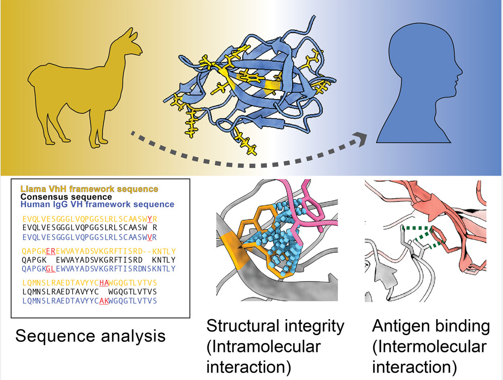
纳米抗体的序列,fasta格式,如:
Nb21
MAQVQLVESGGGLVQAGGSLRLSCAVSGLGAHRVGWFRRAPGKEREFVAAIGANGGNTNYLDSVKGRFTISRDNAKNTIYLQMNSLKPQDTAVYYCAARDIETAEYTYWGQGTQVTVS
输出humanized_data.csv结果文件,包含以下信息:
Position:残基编号
Original AA:原来残基
Humanized?: 是否需要人源化,True表示需要,False表示不需要
Humanized AA: 人源化后的残基
备注:抗体编号方式采用Martin模式。
Llamanade: An open-source computational pipeline for robust nanobody humanization
Sang, Zhe et al. Structure, Volume 30, Issue 3, 418 - 429.e3
https://doi.org/10.1016/j.str.2021.11.006
Nanobodies (Nanobody, Nbs) are a recently emerging class of promising antibody fragments for biomedical and therapeutic applications. Despite its remarkable physicochemical properties, Nbs are derived from camelids and may need to be “humanized” in order to improve translational potential in clinical trials. This module is implemented based on Llamanade, which systematically analyzes the sequence and structural properties of Nbs based on NGS (Next Generation Sequencing) databases and high-resolution structures. A large amount of framework diversity was revealed and key differences between Nbs and human immunoglobulin G (IgG) antibodies were highlighted. Conserved residues that may contribute to improved solubility, structural stability, and antigen binding were identified to facilitate the rational humanization of Nbs. This Module uses Nbs sequence as input to provide information on sequence characterization, model structure, and optimize solutions for Nbs humanization. It takes less than a minute to perform a comprehensive humanization analysis of a given Nbs. It has been successfully applied to humanize a group of structurally diverse and potent SARS-CoV-2 neutralized Nbs.

Nanobody sequence in FASTA format, such as:
Nb21
MAQVQLVESGGGLVQAGGSLRLSCAVSGLGAHRVGWFRRAPGKEREFVAAIGANGGNTNYLDSVKGRFTISRDNAKNTIYLQMNSLKPQDTAVYYCAARDIETAEYTYWGQGTQVTVS
The output csv file (humanized_data.csv) of humanization results includes:
Position: index of residue
Original AA: original residue
Humanized?: need to humanize,0 means no,1 means yes
Humanized AA: residue after humanization
Note: Antibodies are numbered in Martin mode.
Llamanade: An open-source computational pipeline for robust nanobody humanization
Sang, Zhe et al. Structure, Volume 30, Issue 3, 418 - 429.e3
https://doi.org/10.1016/j.str.2021.11.006
该模块基于Smart5UTR模型实现,Smart5UTR 是一种新颖的深度生成模型,设计用于在 mRNA 序列中创建 N1-甲基假尿苷 (m1Ψ) 5’ UTR。Smart5UTR 利用多任务自动编码器框架,利用从大型数据集中学习到的潜在特征,有效地生成 5’ UTR 序列。Smart5UTR设计的mRNA的性能已通过体外和体内实验得到验证。这个强大的工具简化了m1Ψ-5’UTRs的设计,有助于开发更有效的mRNA疗法。

mRNA 5’UTR的序列,如:GGAGCCGAGGCGGGCCGATTCACGATCGGTTCGCAAAAACTGTTTGGGTT
备注:输入序列长度不超过50碱基。
输出result.csv结果文件,包含以下信息:
Original Sequence: 初始序列
Optimized Sequence: 优化后的序列
Optimized MRL: 优化序列预测的MRL值
MRL解释:
mean ribosome load (MRL) 平均核糖体加载值,是反映mRNA序列翻译效率的指标,值越大表示翻译效率越高,一般大于5.0
Xiaoshan Tang, et al., A novel deep generative model for mRNA vaccine development: Designing 5ʹ UTRs with N1-methyl-pseudouridine modification, Acta Pharmaceutica Sinica B, 2023
https://doi.org/10.1016/j.apsb.2023.11.003
Smart5UTR is a novel deep generative model designed for creating N1-methyl-pseudouridine (m1Ψ) 5’ UTRs in mRNA sequences. Utilizing a multi-task autoencoder framework, Smart5UTR efficiently generates 5’ UTR sequences by leveraging the latent features learned from a large dataset. The performance of Smart5UTR-designed mRNA has been validated through in vitro and in vivo experiments. This powerful tool streamlines the design of m1Ψ-5’ UTRs, contributing to the development of more effective mRNA therapeutics.
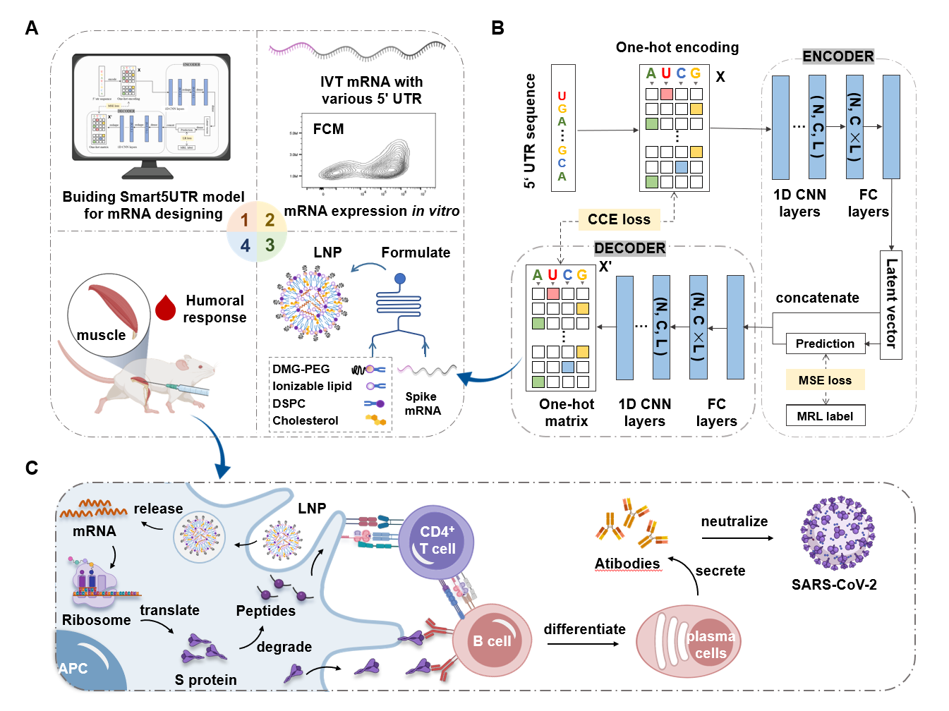
Sequence of mRNA 5’UTR, such as: GGAGCCGAGGCGGGCCGATTCACGATCGGTTCGCAAAAACTGTTTGGGTT
Note: The input sequence length should not exceed 50bp.
The output csv file of optimized sequence includes Original Sequence, Optimized Sequence and Optimized MRL.
MRL is a metric of the average number of ribosomes associated to a given RNA and a proxy for translation efficiency. Higher values indicate higher translation efficiency, generally greater than 5.0
Xiaoshan Tang, et al., A novel deep generative model for mRNA vaccine development: Designing 5ʹ UTRs with N1-methyl-pseudouridine modification, Acta Pharmaceutica Sinica B, 2023
https://doi.org/10.1016/j.apsb.2023.11.003
AlphaMHC v3.0在多个方面相比v2.0进行了大幅优化,
主要包括:
1、风险评分优化,能更好的反映多重HLA激活的风险贡献;
2、引入新的EL和TCR等更多来源的数据,提升了对可递呈表位的预测能力,对TCR分子的支持更好;
3、全新的结果可视化面板(通过WeSeq运行);
为了更好的交互体验和对结果进行可视化,推荐从WeSeq中使用本功能。
测试数据:
从FDA和EMA的临床试验中收集了已知免疫原性的分子及其ADA的分布,使用模型对ADA明显较高(ADA>20%)及较低(ADA<5%)的分子进行分类以测试其预测性能。
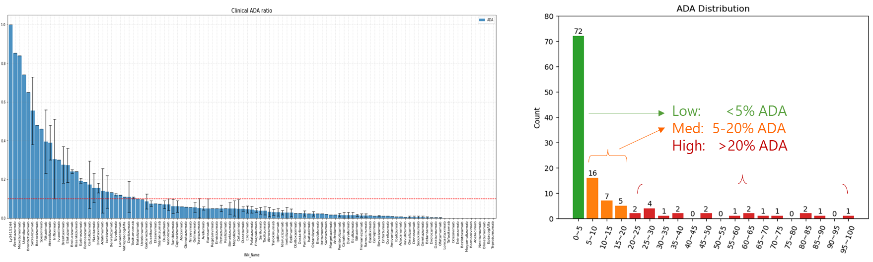
测试结果:
AlphaMHC v3.0全面超越常见算法及v2.0,性能同类最佳(SOTA)
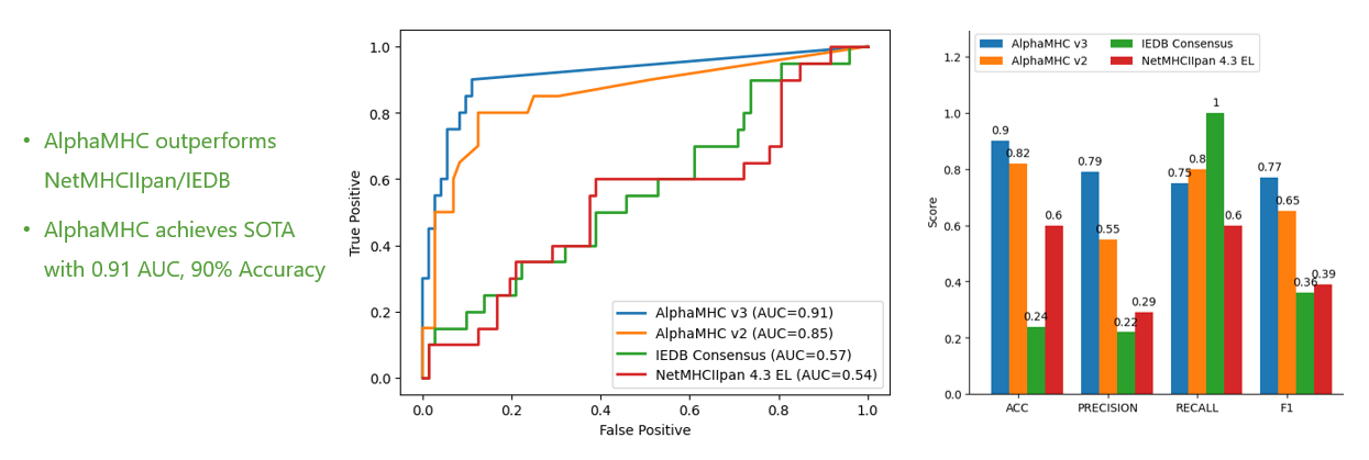
右图中:
计算量消耗
采用阶梯式动态机制,根据提交的序列数量,对应消耗如下:
蛋白序列文件,FASTA格式。支持多条链以及多分子模式。
对于多分子模式,序列名称规则为:分子名.链名,例如:
>mol1.A
XXXXXXX
>mol1.B
XXXXXXX
>mol2.A
XXXXXXX
>mol2.B
XXXXXXX
阈值说明:
当目标蛋白与该分子的评分 ≥ 1 时,将被视为高风险;当评分 < 1 时,将被视为低风险。
Molecule Score 包含以下信息:
| 指标 | 说明 |
|---|---|
| Protein ID | 输入蛋白的名称,如果是多条序列组成的蛋白,会自动合并 |
| Score | 预测的免疫原性风险评分,值越大,风险越高。为所预测短肽的TCE score的求和 |
| Risk | 对应的免疫原性风险等级 |
TCE Score 包含以下信息:
| 指标 | 说明 |
|---|---|
| Protein ID | 所在分子的名称,同个分子的多条序列组成的蛋白会自动合并 |
| Sequence ID | 所在序列的名称 |
| Core_Pos | 表位序列的起始位置 |
| Core | 表位序列(TCE) |
| Score | 表位序列的风险评分,分数越高越可能引起免疫原性。其范围是0-不限 |
| MHC_Count | 可激活的MHC亚型数,考虑了MHC-II的递呈 |
| Tolerance | 免疫耐受的可能性 |
| Germline | 是否存在于人胚系基因中 |
| NextProt | 是否存在于人蛋白组中 |
| OAS | 在NGS人源抗体中出现的频率 |
| TCR | 是否存在于人TCR基因中 |
| LAC | 是否存在于低ADA临床药物(Low ADA CST)中 |
AlphaMHC v3.0 has undergone significant optimizations compared to v2.0 in several aspects, including:
For a better interactive experience and visualization of results, it is recommended to use this feature through WeSeq.
Test Data:
Molecules with known immunogenicity and their ADA distributions collected from clinical trials by the FDA and EMA were used to test the predictive performance of the model on molecules with significantly high ADA (>20%) and low ADA (<5%).
Test Results:
AlphaMHC v3.0 surpasses common algorithms and v2.0 comprehensively, achieving state-of-the-art performance (SOTA).
In the image on the right:
AlphaMHC v3.0 beta Pricing Policy
AlphaMHC v3.0 beta uses a tiered, dynamic pricing model, where charges are calculated based on the number of submitted sequences:
>mol1.A
XXXXXXX
>mol1.B
XXXXXXX
>mol2.A
XXXXXXX
>mol2.B
XXXXXXX
Translation into English:
Molecule Score contains the following information:
| Indicator | Description |
|---|---|
| Protein ID | Name of the input protein; if the protein is composed of multiple sequences, they will be automatically merged |
| Score | Predicted immunogenicity risk score; higher values indicate higher risk. It is the sum of the TCE scores predicted for the peptide |
| Risk | Corresponding immunogenicity risk level |
TCE Score contains the following information:
| Indicator | Description |
|---|---|
| Protein ID | Name of the molecule it belongs to; proteins composed of multiple sequences within the same molecule will be automatically merged |
| Sequence ID | Name of the sequence it belongs to |
| Core_Pos | Starting position of the epitope sequence |
| Core | Epitope sequence (TCE) |
| Score | Risk score of the epitope sequence; higher scores are more likely to cause immunogenicity. The range is from 0 to unlimited |
| MHC_Count | Number of activatable MHC subtypes, considering MHC-II presentation |
| Tolerance | Possibility of immunological tolerance |
| Germline | Whether it exists in human germline genes |
| NextProt | Whether it exists in the human proteome |
| OAS | Frequency of occurrence in NGS-derived human antibodies |
| TCR | Whether it exists in human TCR genes |
| LAC | Whether it exists in Low ADA CST (Low ADA Clinical Study Treatment) medications |
Ramachandran Plots模块是对同源建模后模型质量的评估,仅仅考虑蛋白的构象是否合理,并不涉及能量问题。Ramachandran Plot中φ(phi)表示一个肽单位中α碳左边C-N键的旋转角度, ψ(psi)表示α碳右边C-C键的旋转角度。一般来说落在允许区和最大允许区的氨基酸残基占整个蛋白质的比例高于90%的,可以认为该模型的构象符合立体化学的规则。
蛋白的结构文件,PDB格式。
选择作图链名称,不填默认为all。
图片分辨率(以每英寸点为单位)。
输出结果包括:
| 输出文件名称 | 说明 |
|---|---|
| result_General.png | 通常情况下的拉氏图 |
| result_Glycine.png | 甘氨酸的拉氏图 |
| result_PreProline.png | 脯氨酸前一个残基的拉氏图 |
| result_Proline.png | 脯氨酸的拉氏图 |
图中绿色为最大允许区,浅绿色为允许区,白色为不允许区,青色圆点代表在允许区域的氨基酸,红色圆点代表在不允许区域的氨基酸。在白色区域的氨基酸小于5%时,蛋白结构较为合理。
Sud M. MayaChemTools: An Open Source Package for Computational Drug Discovery. J Chem Inf Model. 2016 Dec 27;56(12):2292-2297.
Lovell SC, Davis IW, Arendall WB 3rd, de Bakker PI, Word JM, Prisant MG, Richardson JS, Richardson DC. Structure validation by Calpha geometry: phi,psi and Cbeta deviation. Proteins. 2003 Feb 15;50(3):437-50.
The Ramachandran Plots module is used to evaluate the quality of models after homology modeling, focusing on the reasonableness of the protein’s conformation without considering energy issues. In a Ramachandran Plot, φ (phi) represents the rotation angle of the C-N bond to the left of the alpha carbon in a peptide unit, and ψ (psi) represents the rotation angle of the C-C bond to the right of the alpha carbon. Generally, if the proportion of amino acid residues falling within the allowed regions and the most favored regions in the Ramachandran Plot is over 90%, the conformation of the model is considered to comply with the rules of stereochemistry.
The output includes:
| Output File Name | Description |
|---|---|
| result_General.png | Ramachandran plot for general residues |
| result_Glycine.png | Ramachandran plot for glycine residues |
| result_PreProline.png | Ramachandran plot for residues before proline |
| result_Proline.png | Ramachandran plot for proline residues |
In the plots, green represents the most favored regions, light green represents allowed regions, white represents disallowed regions, cyan dots represent amino acids in allowed regions, and red dots represent amino acids in disallowed regions. When the percentage of amino acids in the white region is less than 5%, the protein structure is considered reasonable.
Therapeutic Antibody Profiler (TAP) 基于抗体可变区的结构计算抗体的可开发性性质。TAP目前支持单抗与纳米抗体的性质计算。
对于单抗计算以下5个性质,以确定输入单抗的可开发性指标是否与临床阶段的单抗的属性相匹配:
针对851的治疗性单体(临床I期及之后)的Fv区计算的可开发性指标范围如下(最新更新日期为2025年2月24日):
| Property | Amber Region | Red Region |
|---|---|---|
| Total CDR Length (L) | 37 ≤ L ≤ 42 | L < 37 |
| 55 ≤ L ≤ 65 | L > 65 | |
| Patches of Surface Hydrophobicity (PSH) | 95.77 ≤ PSH ≤ 111.40 | PSH < 95.77 |
| 167.64 ≤ PSH ≤ 211.65 | PSH > 211.65 | |
| Patches of Positive Charge (PPC) | 1.34 ≤ PPC ≤ 4.20 | PPC > 4.24 |
| Patches of Negative Charge (PNC) | 1.99 ≤ PNC ≤ 4.43 | PNC > 5.67 |
| Structural Fv Charge Symmetry Parameter (SFvCSP) | -30.60 ≤ SFvCSP ≤ -6.00 | SFvCSP < -30.60 |
Amber Region: 指标在851个治疗性抗体(临床I期及之后)的Fv区计算的指标范围内,属于合理区域
Red Region:指标不合理区域,需要调整
Amber Region和Red Region的区域范围定义如下表所示。
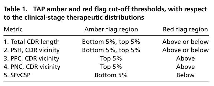
对于纳米抗体,计算6个性质,以确定输入纳米抗体的可开发性指标是否与临床阶段的纳米抗体的属性相匹配:
针对36的治疗性纳米抗体(临床I期及之后)计算的可开发性指标范围如下(最新更新日期为2025年8月14日):
| Property | Amber Region | Red Region |
|---|---|---|
| Total CDR Length (L) | 20 ≤ L ≤ 24 | L < 20 |
| 38 ≤ L ≤ 39 | L > 39 | |
| CDR3 Length (L) | 5 ≤ L ≤ 8 | L < 5 |
| 22 ≤ L ≤ 23 | L > 23 | |
| CDR3 Compactness (CC) | 0.56 ≤ CC ≤ 0.81 | PSH < 0.56 |
| 1.57 ≤ CC ≤ 1.61 | CC > 1.61 | |
| Patches of Surface Hydrophobicity (PSH) | 73.40 ≤ PSH ≤ 79.59 | PSH < 73.40 |
| 126.83 ≤ PSH ≤ 155.47 | PSH > 155.47 | |
| Patches of Positive Charge (PPC) | 0.39 ≤ PPC ≤ 1.18 | PPC > 1.18 |
| Patches of Negative Charge (PNC) | 1.47 ≤ PNC ≤ 1.88 | PNC > 1.88 |
Amber Region 与 Red Region的定义同上。
抗体结构文件,支持单抗或纳米抗体,PDB格式
多个单抗Fv结构或者多个纳米抗体结构(PDB格式)的压缩文件,压缩文件格式支持zip,tar或tar相关的压缩格式(.tar.gz, .bz2, .xz)
当同时上传单一结构和压缩包时会合并计算。
当选择该选项时,进行纳米抗体的类TAP计算。默认情况下计算抗体的TAP。
输出打分文件,CSV格式,默认为score.csv。
输出每个残基的打分,CSV格式,默认为detail.csv。
输出打分文件score.csv,输出以下信息:
Total CDR Length:CDR区域氨基酸长度
CDR3 Length:CDR3长度(纳米抗体时输出)
CDR3 Compactness:CDR3紧凑度(纳米抗体时输出)
CDR Vicinity PSH Score (Kyte & Doolittle):CDR区域及其周围的表面疏水性程度
CDR Vicinity PPC Score:CDR区域及其周围的表面正电荷程度
CDR Vicinity PNC Score:CDR区域及其周围的表面负电荷程度
SFvCSP Score:Fv区的重、轻链之间的净电荷失衡程度(单抗时输出)
输出每个残基的打分文件detail.csv,输出以下信息:
PDBFile:结构文件名称
ChainType:链名(单抗时输出)
ResIndex:残基编号
ResLabel:残基名称
CDR Vicinity PSH Score (Kyte & Doolittle):残基的PSH分数
CDR Vicinity PPC Score:残基的PPC分数
CDR Vicinity PNC Score:残基的PNC分数
The Therapeutic Antibody Profiler (TAP) compares your antibody variable domain sequence against multiple developability guidelines derived from clinical-stage therapeutic values. TAP currently supports property calculations for both monoclonal antibodies and nanobodies.
For monoclonal antibodies, the following five properties are calculated to see if your antibody design is commenserate with those of clinical-stage therapeutics:
The TAP Guidelines were last updated on 24th February 2025:
| Property | Amber Region | Red Region |
|---|---|---|
| Total CDR Length (L) | 37 ≤ L ≤ 42 | L < 37 |
| 55 ≤ L ≤ 65 | L > 65 | |
| Patches of Surface Hydrophobicity (PSH) | 95.77 ≤ PSH ≤ 111.40 | PSH < 95.77 |
| 167.64 ≤ PSH ≤ 211.65 | PSH > 211.65 | |
| Patches of Positive Charge (PPC) | 1.34 ≤ PPC ≤ 4.20 | PPC > 4.24 |
| Patches of Negative Charge (PNC) | 1.99 ≤ PNC ≤ 4.43 | PNC > 5.67 |
| Structural Fv Charge Symmetry Parameter (SFvCSP) | -30.60 ≤ SFvCSP ≤ -6.00 | SFvCSP < -30.60 |
Amber Region: Within the reasonable region of 851 post Phase-I therapeutic Fvs
Red Region: Unreasonable region, the developability needs to be optimized
The following table defines the scope of Amber Region and Red Region.

For nanobodies, six properties are calculated to determine whether the developability profile of the input nanobody matches the attributes of clinical-stage nanobodies:
The developability ranges derived from 36 therapeutic nanobodies (Phase I and beyond) are as follows (last updated: 14 August 2025):
| Property | Amber Region | Red Region |
|---|---|---|
| Total CDR Length (L) | 20 ≤ L ≤ 24 | L < 20 |
| 38 ≤ L ≤ 39 | L > 39 | |
| CDR3 Length (L) | 5 ≤ L ≤ 8 | L < 5 |
| 22 ≤ L ≤ 23 | L > 23 | |
| CDR3 Compactness (CC) | 0.56 ≤ CC ≤ 0.81 | PSH < 0.56 |
| 1.57 ≤ CC ≤ 1.61 | CC > 1.61 | |
| Patches of Surface Hydrophobicity (PSH) | 73.40 ≤ PSH ≤ 79.59 | PSH < 73.40 |
| 126.83 ≤ PSH ≤ 155.47 | PSH > 155.47 | |
| Patches of Positive Charge (PPC) | 0.39 ≤ PPC ≤ 1.18 | PPC > 1.18 |
| Patches of Negative Charge (PNC) | 1.47 ≤ PNC ≤ 1.88 | PNC > 1.88 |
The definition of Amber Region and Red Region are same as above.
Antibody Structure file in PDB format, both monoclonal antibodies and nanobodies are supported.
A single compressed archive (zip, tar, or any tar-based format such as .tar.gz, .bz2, .xz) that contains multiple monoclonal-antibody Fv structures or multiple nanobody structures in PDB format.
When a single structure file and an archive are uploaded simultaneously, the calculations will be merged.
When this option is selected, a TAP-like calculation is performed for nanobodies. By default, TAP is calculated for antibodies.
Output score file in CSV format, default is score.csv.
Output score file of each residue in CSV format, default is detail.csv.
Outputs a summary file named score.csv containing:
Also outputs a per-residue file named detail.csv containing:
IgG Modeling对抗体全长序列进行建模,用于构建抗体IgG完整的三维结构,支持单特异性和双特异性抗体。
自动识别全长序列中的可变区(Fv)序列并通过SOTA的方法(目前为ESMFold)进行建模,IgG的其余部分包括Fc和linker以已知全长抗体的晶体结构为模板通过空间约束条件进行同源模建,效果比直接用AF2等方法预测完整IgG结构更优。
抗体的第一条重链的序列。
抗体的第一条轻链的序列。
抗体的第二条重链的序列,非必填,仅在双抗建模时输入。
抗体的第二条轻链的序列,非必填,仅在双抗建模时输入。
IgG亚型,目前支持IgG1和IgG4两种类型。
注意:
1)当待建模序列为单抗时,只需要写入H1与L1即可,H1与H2相同,L1与L2相同,最终模型包含2条相同的重链和2条相同的轻链。
2)当待建模序列为双抗时,需要输入四条链的序列,最终模型包含2条不同重链和2条不同轻链。
输出结果包括:
| 输出文件名称 | 说明 |
|---|---|
| antibody_001.pdb-antibody_003.pdb | 输出三个抗体全长的结构 |
| scores.csv | 抗体全长结构打分,其中Spatial Restraint Penalty (SRP)是对结构构象约束的惩罚评分,数值越低代表违反的空间约束越少,越推荐使用。 |
IgG Modeling is used to model the full-length sequence of antibodies to construct the complete three-dimensional structure of antibody IgG, supporting both monospecific and bispecific antibodies. It automatically identifies the variable region (Fv) sequence in the full-length sequence and models it using state-of-the-art methods (currently ESMFold). The remaining parts of IgG, including Fc and linker, are modeled homologously based on the crystal structure of known full-length antibodies as templates, using spatial constraints, which yields better results compared to directly predicting the complete IgG structure using methods like AF2.
The output includes:
| Output File Name | Description |
|---|---|
| antibody_001.pdb-antibody_003.pdb | Structures of three full-length antibodies |
| scores.csv | Scoring of the full-length antibody structures, Among them, Spatial Restraint Penalty (SRP) is a penalty score for conformational restraints on the structure. Lower values indicate fewer violated spatial restraints and are more recommended for use. |
Substructure Search模块是小分子子结构搜索模块,实现在化合物库中查询出含有特定子结构的分子并输出到SDF文件中。子结构搜索是化学信息学研究中的常用操作,也可以用于虚拟筛选,从小分子商业库中搜索出含有特定功能片段的分子用于后续实验验证。
搜索子结构文件,SDF或者SMI格式
通过WeDraw界面画模板小分子,只允许单个小分子。
搜索子结构SMILES字符,例如
c1ccccc1
CC(N)=O
选择用于相似性搜索的分子库,该模块提供17个公共分子数据库用于进行相似性搜索:
提示说明:Public Library与Private Library选填其中一个。
用于搜索的个人分子库,仅支持SDF格式。
提示说明:Public Library与Private Library选填其中一个。
输出文件名称,默认matched_molecules.sdf。
结果文件为分子库中含有子结构的化合物matched_molecules.sdf。
Public Library与Private Library选填其中一个。
用于搜索的个人分子库,仅支持SDF格式。
Public Library与Private Library选填其中一个。
输出文件名称,默认matched_molecules.sdf。
结果文件为分子库中含有子结构的化合物matched_molecules.sdf。
The Substructure Search module is a tool for searching for specific substructures within a compound library and outputting them to an SDF file. Substructure searching is a common operation in cheminformatics research and can be used for virtual screening to identify molecules in commercial small molecule libraries containing specific functional fragments for subsequent experimental validation.
File containing the substructure to search for, in SDF or SMI format.
Draw a template small molecule using the WeDraw interface, allowing only a single small molecule.
SMILES string of the substructure to search for, for example:
c1ccccc1
CC(N)=O
Select the public molecular library for the substructure search module, which provides 16 public molecular databases for substructure searching.
Personal molecular library for searching, supporting SDF format.
Note: Choose either Public Library or Private Library.
Name of the output file, default is matched_molecules.sdf.
The result file contains compounds from the compound library that contain the specified substructure, saved as matched_molecules.sdf.
Small Molecule Minimization是针对小分子结构进行能量最小化优化并得到优化后的3D结构。支持UFF和MMFF两种分子力场,支持SDG, ETDG, KDG, ETKDG四种构象采样方法,用于生成初始3D构象。注意,每个分子只输出一个能量最低构象,构象搜索推荐使用 3D Conf (AlphaConf)模块。
小分子文件,支持Mol (.mol), SD (.sdf, .sd), SMILES (.smi .csv, .tsv, .txt)。
输出文件名称,仅支持SDF格式,默认为minimized_struture.sdf。
3D构象方法:SDG, ETDG, KDG, ETKDG, None.
用于能量最小化的力场方法,包括UFF(Universal Force Field)和MMFF(Merck Molecular Mechanics Force Field)。
使用并行计算。
在基于力场优化期间针对每个分子执行的最大迭代次数,默认500。
随机数,用于重现优化后的结构。
得到能量最小化后的小分子3D结构文件minimized_struture.sdf。
Sud M. MayaChemTools: An Open Source Package for Computational Drug Discovery. J Chem Inf Model. 2016 Dec 27;56(12):2292-2297.
Riniker, S.; Landrum, G. A. Better informed distance geometry: Using what we know to improve conformation generation. JCIM. 2015, 55, 2562-2574.
Rappe, A.K.; Casewit, C.J.; Colwell, K.S.; Goddard III, W.A.; Skiff, W.M. UFF, a full periodic table force field for molecular mechanics and molecular dynamics simulations. J. Am. Chem. Soc. 1992, 114, 10024-10035.
Halgren, T.A.; Merck Molecular Force Field. I. Basis, Form, Scope, Parameterization, and Performance of MMFF94. 1996, J. Comput. Chem., 17, 490-519.
Halgren, T.A.; Merck molecular force field. V. Extension of MMFF94 using experimental data, additional computational data, and empirical rules. J. Compt. Chem. 1996, 17, 616-641.
Small Molecule Minimization is a tool module designed to perform energy minimization optimization on small molecule structures and obtain the optimized 3D structure. It supports two molecular force fields, UFF and MMFF, as well as four conformation sampling methods: SDG, ETDG, KDG, and ETKDG, used to generate initial 3D conformations. Note that only one energy-minimized conformation is output for each molecule, and for conformational search, it is recommended to use the 3D Conf (AlphaConf) module.
Input file for the small molecule, supporting Mol (.mol), SD (.sdf, .sd), SMILES (.smi .csv, .tsv, .txt) formats.
Name of the output file, only supports SDF format, default is minimized_structure.sdf.
3D conformation method: SDG, ETDG, KDG, ETKDG, None.
Force field method for energy minimization, including UFF (Universal Force Field) and MMFF (Merck Molecular Mechanics Force Field).
Utilize parallel computing.
Maximum number of iterations performed for each molecule during force field optimization, default is 500.
Random number used to reproduce the optimized structure.
Obtain the energy-minimized 3D structure file for the small molecule as minimized_structure.sdf.
PDB ReNumbering是针对蛋白残基重新编号的工具模块,同时支持抗体kabat,imgt以及chothia的重编号。输入蛋白结构PDB文件,输出重新编号后的PDB文件。
输入蛋白结构文件,PDB格式。
重编号类型,支持指定链从指定数字开始编号,同时支持抗体结构重新编号。
numeric:氨基酸序号重编号
kabat:抗体kabat编号规则重编号
imgt:抗体imgt编号规则重编号
chothia:抗体chothia编号规则重编号
链名,指定具体的链名进行重编号操作。支持输入多条链名,链名之间用英文逗号“,”隔开,如“H,L”。
针对氨基酸序号重编号,指定起始编号数字。
重编号后的文件名称。
重编号后的结构文件名称,默认输出renumbering.pdb。
注意:如果输入是抗体结构,输出结构中重链的链名会自动改为H,轻链链名会改为L。
PDB ReNumbering is a tool module for renumbering protein residues, supporting renumbering according to the kabat, imgt, and chothia numbering schemes for antibodies. Input a protein structure PDB file and get the renumbered PDB file as output.
Input protein structure file in PDB format.
Renumbering type, supports starting numbering from a specified number for a specific chain, and also supports renumbering for antibody structures.
Chain name, specifies the chain to perform renumbering.Support multiple chain names as input, separated by commas, e.g., “H,L”.
For renumbering amino acid residues numerically, specifies the starting number.
Name of the renumbered file.
The renumbered structure file is named by default as renumbering.pdb.
Note: If the input is an antibody structure, the chain names in the output structure will be automatically changed to H for the heavy chain and L for the light chain.
AC2SDF模块是一个格式转换工具,用于将AlphaConf模块生成的构象压缩二进制文件AC.GZ转为便于查看结构的SDF文件。
输入构象文件,AC.GZ格式,由AlphaConf模块生成
片段库文件,AUX.GZ格式,由AlphaConf模块生成
转换生成的SDF文件名称
| 输出文件名称 | 说明 |
|---|---|
| ligands_confs.sd | 转换生成的SDF文件,可通过WeView直接查看构象 |
The AC2SDF module is a format conversion tool used to convert the compressed binary conformation file AC.GZ generated by the AlphaConf module into an SDF file for easier visualization of the structure.
Input conformation file in AC.GZ format generated by the AlphaConf module.
Fragment library file in AUX.GZ format generated by the AlphaConf module.
Name of the converted SDF file.
| Output File Name | Description |
|---|---|
| ligands_confs.sd | Converted SDF file that can be viewed directly using WeView for conformation visualization. |

Sequence Mutation是蛋白序列突变模块,用于针对特定位点批量生成突变序列,支持多样的突变策略,包括设定不同的突变位置及突变类型。
突变策略包括:
突变类型支持:
蛋白原始序列或者fasta格式的序列
突变位点,支持多个位点,英文逗号分割,例如:2,3
突变类型,支持三种类型:Ala 丙氨酸突变,His 组氨酸突变,Sat 饱和突变
链名,输出突变信息时加上指定链名
生成突变序列的文件名称,FASTA格式
蛋白突变信息文件,TXT格式
蛋白原始序列或者fasta格式的序列
同源序列,一般由序列比对产生的结果文件,FASTA 格式
序列比对的方法,mafft或者muscle
频数截断值,大于截断值的氨基酸才会选择作为突变目标
链名,输出突变信息时加上指定链名
生成突变序列的文件名称,FASTA格式
蛋白突变信息文件,TXT格式
蛋白原始序列或者fasta格式的序列
抗体CDR编号规则:kabat, imgt, chothia
突变类型,支持三种类型:Ala 丙氨酸突变,His 组氨酸突变,Sat 饱和突变
链名,输出突变信息时加上指定链名
生成的包含蛋白突变序列的文件名称,FASTA格式
生成的包含蛋白突变信息的文件名称,TXT格式
蛋白原始序列或者fasta格式的序列
抗体CDR编号规则:kabat, imgt, chothia
同源序列,一般由序列比对产生的结果文件,FASTA 格式
序列比对的方法,mafft或者muscle
频数截断值,大于截断值的氨基酸才会选择作为突变目标
链名,输出突变信息时加上指定链名
生成的包含蛋白突变序列的文件名称,FASTA格式
生成的包含蛋白突变信息的文件名称,TXT格式
| 输出文件名称 | 说明 |
|---|---|
| mutants.fasta | 生成突变序列的文件名称,FASTA格式 |
| mutations.txt | 蛋白突变信息文件,TXT格式,每行一个突变记录,例如:Q2A 代表第2位氨基酸Q突变为氨基酸A |
Sequence Mutation is a protein sequence mutation module that allows for batch generation of mutated sequences at specific positions, supporting various mutation strategies including setting different mutation positions and types.
Mutation strategies include:
Supported mutation types include:
Original protein sequence or sequence in FASTA format.
Mutation positions, support for multiple positions separated by commas, e.g., 2,3.
Mutation types, supporting three types: Ala (Alanine mutation), His (Histidine mutation), Sat (Saturation mutation).
Chain name to be included in the mutation information output.
File name for generated mutated sequences in FASTA format.
Protein mutation information file in TXT format.
Original protein sequence or sequence in FASTA format.
Homologous sequences, typically generated from sequence alignment results in FASTA format.
Alignment methods for sequence alignment: mafft or muscle.
Frequency cutoff value, only amino acids with frequencies greater than the cutoff value will be selected as mutation targets.
Chain name to be included in the mutation information output.
File name for generated mutated sequences in FASTA format.
Protein mutation information file in TXT format.
Original protein sequence or sequence in FASTA format.
Antibody CDR numbering rule: kabat, imgt, chothia.
Mutation types, supporting three types: Ala (Alanine mutation), His (Histidine mutation), Sat (Saturation mutation).
Chain name to be included in the mutation information output.
File name for generated mutated protein sequences in FASTA format.
File name for generated protein mutation information in TXT format.
Original protein sequence or sequence in FASTA format.
Antibody CDR numbering rule: kabat, imgt, chothia.
Homologous sequences, typically generated from sequence alignment results in FASTA format.
Alignment methods for sequence alignment: mafft or muscle.
Frequency cutoff value, only amino acids with frequencies greater than the cutoff value will be selected as mutation targets.
Chain name to be included in the mutation information output.
File name for generated mutated protein sequences in FASTA format.
File name for generated protein mutation information in TXT format.
| Output File Name | Description |
|---|---|
| mutants.fasta | File name for generated mutated sequences in FASTA format. |
| mutations.txt | Protein mutation information file in TXT format, with each line representing a mutation record, e.g., Q2A represents the mutation of amino acid Q at position 2 to amino acid A. |
MD Distance是针对分子动力学轨迹的距离分析模块,输出两个组之间距离 (质心距离或几何中心距离) 随时间的变化情况。自定义组别时需要注意,如果只需测量两个原子之间的距离则填写Custom Atom1和Custom Atom2即可;当同时填写Custom Resid1和Custom Atom1时,组别1的原子数是Custom Atom1与Custom Resid1交集的原子。
MD模拟后得到的路径文件,可以在GMX MD Run (GMX2023)模块或者AlphaAutoMD (GMX2023)模块中获取。
选择需要计算的组别1:Protein,DNA,RNA。
可以根据PDB中小分子的名称填写组别名称。
选择需要计算的组别1:Protein,DNA,RNA。
可以根据PDB中小分子的名称填写组别名称。
自定义需要计算的组1残基编号,连续参数可用“-”表示,不连续残基用逗号隔开,例如:1-10,15。自定义组别之间是并集。
自定义需要计算的组1原子编号,连续参数可用“-”表示,不连续原子用逗号隔开,例如:1-10,15。自定义组别之间是并集。
自定义需要计算的组2残基编号,连续参数可用“-”表示,不连续残基用逗号隔开,例如:1-10,15。自定义组别之间是并集。
自定义需要计算的组2原子编号,连续参数可用“-”表示,不连续原子用逗号隔开,例如:1-10,15。自定义组别之间是并集。
每一帧的间隔时间(单位ns)。
输出结果包括:
| 输出文件名称 | 说明 |
|---|---|
| dist.csv | 距离分析CSV文件 |
| dist.xvg | 距离分析XVG文件 |
| dist.png | 距离分析PNG文件 |
其中dist.csv包括信息如下:
| 字段名称 | 说明 |
|---|---|
| Time (ns) | 时间 |
| Distance (nm) | 组别之间的距离 |
MD Distance is a distance analysis module for molecular dynamics trajectories, providing the variation of distance (center-of-mass distance or geometric center distance) between two groups over time. When defining custom groups, it is important to note that if you only need to measure the distance between two atoms, you can fill in Custom Atom1 and Custom Atom2. When both Custom Resid1 and Custom Atom1 are filled in, the number of atoms in group 1 is the intersection of Custom Atom1 and Custom Resid1.
Path file obtained after MD simulation, available in the GMX MD Run (GMX2023) module or AlphaAutoMD (GMX2023) module.
Select the group 1 for calculation: Protein, DNA, RNA.
You can enter the group name based on the name of the small molecule in the PDB.
Select the group 2 for calculation: Protein, DNA, RNA.
You can enter the group name based on the name of the small molecule in the PDB.
Custom residue numbers for group 1 that need to be calculated. Use “-” for continuous parameters and separate non-continuous residues with commas, for example: 1-10,15. Custom groups are unions of specified residues.
Custom atom numbers for group 1 that need to be calculated. Use “-” for continuous parameters and separate non-continuous atoms with commas, for example: 1-10,15. Custom groups are unions of specified atoms.
Custom residue numbers for group 2 that need to be calculated. Use “-” for continuous parameters and separate non-continuous residues with commas, for example: 1-10,15. Custom groups are unions of specified residues.
Custom atom numbers for group 2 that need to be calculated. Use “-” for continuous parameters and separate non-continuous atoms with commas, for example: 1-10,15. Custom groups are unions of specified atoms.
Time interval for each frame (in ns).
The output includes:
| Output File Name | Description |
|---|---|
| dist.csv | Distance analysis CSV file |
| dist.xvg | Distance analysis XVG file |
| dist.png | Distance analysis PNG file |
The dist.csv file includes the following information:
| Field Name | Description |
|---|---|
| Time (ns) | Time |
| Distance (nm) | Distance between the groups |
Peptide VS模块集成了AutoDock Vina与AutoDock CrankPep进行蛋白-多肽的分子对接,从而预测蛋白-多肽的构象、得到分子对接的能量以及结合亲和力。AutoDock CrankPep则是一个专门用于多肽对接工具,其基于蛋白折叠和刚性受体网格能量背景下,采用蒙特卡罗方法对多肽的折叠进行计算,产生多肽的对接构象。
受体结构文件,PDB格式。
多肽的氨基酸序列,可以成功对接长度达20个氨基酸的肽。一行一条序列,例如:
AINMDSFHTWKVLECGRPQY
HRIAQCSDKW
IYSADCLPKG
AAAAIS
注意:最多支持多肽的氨基酸序列长度为35左右。
对接口袋中心的三维坐标(XYZ),空格分割。例如:10 2 -11。
对接口袋长方体盒子的大小,必须是整数,空格分割,例如 30 30 30。
每个多肽与蛋白对接后输出的构象数目,默认为10。
输出结果包括:
| 输出文件名称 | 说明 |
|---|---|
| Scores.csv | 提交多肽与受体的打分文件。 |
| output_complex_top1.pdb | 展示打分第一的多肽与受体的复合物构象。 |
| output_complex_topn.tar.gz | TopN多肽“Out Pose”构象数与受体形成的复合物结构PDB文件压缩包。 |
其中Scores.csv包括信息如下:
| 字段名称 | 说明 |
|---|---|
| Name | 对接多肽名称 |
| Score(kcal/mol) | 对接打分,该值越低说明结合亲和力越高。 |
| Cluster RMSD | 聚类后,构象之间的RMSD |
| Average RMSD | 平均RMSD |
| Complex File Name | 复合物文件名称 |
The Peptide VS module integrates AutoDock Vina and AutoDock CrankPep for protein-polypeptide molecular docking, predicting the conformation of protein-polypeptide complexes, docking energy, and binding affinity. AutoDock Vina is a molecular docking tool that compares the binding affinities between multiple molecules, used for screening, designing, and optimizing drug molecules. AutoDock CrankPep is a specialized tool for peptide docking that uses a Monte Carlo method to calculate peptide folding based on protein folding and rigid receptor grid energy background, generating docking conformations for peptides. This module has been successfully demonstrated to redock peptides of up to 20 amino acids in length.
Structure file of the receptor in PDB format.
The peptide amino acid sequences can be successfully docked for peptides up to 20 amino acids in length.
Each line should contain one sequence, for example:
AINMDSFHTWKVLECGRPQY
HRIAQCSDKW
IYSADCLPKG
AAAAIS
Note: The maximum supported peptide amino acid sequence length is approximately 35.
Three-dimensional coordinates (XYZ) of the docking pocket center, separated by spaces. For example: -44.497 -22 -5.
Size of the docking pocket rectangular box, must be integers, separated by spaces, for example 30 30 30.
Specify the top N small molecules for scoring as output files, default is 100.
Number of conformations output for each peptide-protein docking, default is 10.
The output includes:
| Output File Name | Description |
|---|---|
| Scores.csv | Scoring file for the docking of peptides with the receptor. |
| output_complex_top1.pdb | Conformation of the top scoring peptide-receptor complex. |
| output_complex_topn.tar.gz | Compressed PDB files of the top N peptide “Out Pose” conformations forming complexes with the receptor. |
The Scores.csv file includes the following information:
| Field Name | Description |
|---|---|
| Name | Name of the docked peptide |
| Score(kcal/mol) | Docking score, lower values indicate higher binding affinity. |
| Complex File Name | Name of the complex file |
Alanine Scan (MMPBSA)是计算丙氨酸突变后的结合自由能,并且提供能量分解数据、结合常数(Ka)、抑制剂常数(Ki)。熵的计算采用的是张增辉教授的相互作用熵的方法,该方法直接从分子动力学模拟计算结合自由能的熵组分(相互作用熵或-TΔS),但是需要选取结构稳定部分进行计算。
本模块提供四种计算方法,其中 Trajectory 是针对进行分子动力学模拟轨迹后计算其受配体之间的结合自由能;One Structure 是针对一帧pdb结构或者对接得到的PDB结构计算受配体之间的结合自由能,MMPBSA of One Structure 计算流程中可以直接输入PDB进行计算。
Index Name 是输入受配体组别名称;Custom Name 则是输入受配体的在PDB中的残基编号。
MD模拟后得到的路径文件,可以在GMX MD Run (GMX2023)模块或者AlphaAutoMD模块中获取。
受体名称,可以为Protein、DNA、RNA。
配体名称,可以为Protein、DNA、RNA。如果为小分子,填写其在PDB中的名称。如果体系中除了蛋白以外为配体(包括小分子)可用Other表示。
突变扫描为丙氨酸(ALA)的氨基酸位置。格式为res1:res2:res3:res4,其中“res1-res4”数字为残基编号。
丙氨酸扫描时使用的力场。
起始帧时间,单位ps。最好选取RMSD稳定时区进行计算,以消除结构不稳定时导致的整体熵偏大。
结束帧时间,单位ps。最好选取RMSD稳定时区进行计算,以消除结构不稳定时导致的整体熵偏大。
间隔时间,单位ps。
索引文件,ndx格式。当体系中存在膜结构的时候可以通过Membrane Solvation模块获取index.ndx文件。膜模拟中的受体为receptor,配体为ligand,膜为membrane。只能是AMBER力场下构建的膜体系才能进行计算。
定义受体组别进行结合能计算。组别中填写的为蛋白氨基酸或者核酸碱基的序号。例如1-213或者1-211,212-213。蛋白氨基酸或者核酸碱基序号从1开始重新编号,与初始pdb氨基酸编号无关。
定义配体组别进行结合能计算。组别中填写的为蛋白氨基酸或者核酸碱基的序号。例如1-213或者1-211,212-213。蛋白氨基酸或者核酸碱基序号从1开始重新编号,与初始pdb氨基酸编号无关。
拓扑文件,由MD Solvation模块或者Membrane Solvation模块得到。
结构文件,.gro格式,由MD Solvation模块或者Membrane Solvation模块得到。
体系参数压缩文件,tar.gz格式。由MD Solvation模块或者Membrane Solvation模块得到。
输出结果包括:
| 输出文件名称 | 说明 |
|---|---|
| MMPBSA_result.txt | MMPBSA丙氨酸突变结果汇总文件。 |
| MMPBSA_Residue.csv | 丙氨酸突变能量分解数据CSV文件。 |
| MMPBSA.pdb | 丙氨酸突变后,原子对应的MMPBSA能量放到PDB文件。可以做对应能量类别的表面图,从图的颜色深浅可以看出哪些区域对结合能贡献值较大。 |
| MMPBSA.tar.gz | MMPBSA所有原始文件。包括_mmpbsa_residue_#.txt是每个残基对应的每个能量类别的数值,共包含7个能量类别:范德华能(VDW)、静电能(ELE)、溶剂化能极性部分(PB)、溶剂化能非极性部分(SA)、VDW+ELE=MM、PB+SA=PBSA、MM+PBSA=Binding/MMPBSA。_mmpbsa_residue.txt是对上述7个文件的总结,即为MMPBSA_Residue.csv对应的原始文件。_mmpbsa_atom#.pdb是将每个原子对应的能量类别放到pdb文件,与MMPBSA.pdb相似。 |
GROMACS: High performance molecular simulations through multi-level parallelism from laptops to supercomputers. M. J. Abraham, T. Murtola, R. Schulz, S. Páll, J. C. Smith, B. Hess, E. Lindahl, SoftwareX, 1, (2015), 19-25.
Duan L, Liu X, Zhang JZ. Interaction Entropy: A New Paradigm for Highly Efficient and Reliable Computation of Protein-Ligand Binding Free Energy. J Am Chem Soc. 2016 May 4;138(17):5722-8.
https://github.com/Electrostatics/apbs/blob/main/docs/index.rst
Alanine Scan (MMPBSA) calculates the binding free energy after alanine mutations and provides energy decomposition data, binding constants (Ka), and inhibitor constants (Ki). The entropy calculation uses the method of interaction entropy proposed by Professor Zhang Zenghui, which directly calculates the entropy component of the binding free energy (interaction entropy or -TΔS) from molecular dynamics simulations, but requires selecting stable structural regions for calculation. This module provides four calculation methods. Among them, Trajectory calculates the binding free energy between the receptor and ligand after molecular dynamics simulation trajectories; One Structure calculates the binding free energy between the receptor and ligand for a single frame PDB structure or a docked PDB structure; MMPBSA of One Structure allows direct input of a PDB for calculation. Index Name is the input receptor-ligand group name, while Custom Name is the input residue numbers of the receptor-ligand in the PDB.
Path file obtained after MD simulation, available in the GMX MD Run (GMX2023) module or AlphaAutoMD module.
Name of the receptor, can be Protein, DNA, or RNA.
Name of the ligand, can be Protein, DNA, or RNA. If it is a small molecule, enter its name in the PDB. Use ‘Other’ if the system contains a ligand (including small molecules) other than proteins.
Amino acid positions where mutations to alanine (ALA) are scanned. The format is res1:res2:res3:res4, where “res1-res4” are residue numbers.
Force field used for alanine scanning.
Start frame time in ps. It is best to select a stable RMSD region for calculation to eliminate large overall entropy caused by structural instability.
End frame time in ps. It is best to select a stable RMSD region for calculation to eliminate large overall entropy caused by structural instability.
Time interval in ps.
Index file in ndx format. When there is a membrane structure in the system, you can obtain the index.ndx file through the Membrane Solvation module. In membrane simulations, the receptor is ‘receptor’, the ligand is ‘ligand’, and the membrane is ‘membrane’. Only membrane systems built under the AMBER force field can be calculated.
Define receptor groups for binding energy calculation. Enter the sequence numbers of protein amino acids or nucleic acid bases in the group. For example, 1-213 or 1-211,212-213. Protein amino acid or nucleic acid base numbers start from 1 and are independent of the initial pdb amino acid numbering.
Define ligand groups for binding energy calculation. Enter the sequence numbers of protein amino acids or nucleic acid bases in the group. For example, 1-213 or 1-211,212-213. Protein amino acid or nucleic acid base numbers start from 1 and are independent of the initial pdb amino acid numbering.
Topology file obtained from the MD Solvation module or Membrane Solvation module.
Structure file in .gro format obtained from the MD Solvation module or Membrane Solvation module.
System parameter compression file in tar.gz format. Obtained from the MD Solvation module or Membrane Solvation module.
The output includes:
| Output File Name | Description |
|---|---|
| MMPBSA_result.txt | Summary file of MMPBSA alanine mutation results. |
| MMPBSA_Residue.csv | Energy decomposition data for alanine mutations in CSV format. |
| MMPBSA.pdb | MMPBSA energy corresponding to atoms after alanine mutations in a PDB file. This can be used to create a surface map of energy categories, where the color depth indicates the regions contributing significantly to the binding energy. |
| MMPBSA.tar.gz | All original MMPBSA files. Includes mmpbsa_residue#.txt which contains the values of each energy category for each residue, totaling 7 energy categories: van der Waals energy (VDW), electrostatic energy (ELE), polar part of solvation energy (PB), nonpolar part of solvation energy (SA), VDW+ELE=MM, PB+SA=PBSA, MM+PBSA=Binding/MMPBSA. _mmpbsa_residue.txt is a summary of the above 7 files, corresponding to the original file MMPBSA_Residue.csv. _mmpbsa_atom#.pdb assigns the energy categories to each atom in a pdb file, similar to MMPBSA.pdb. |
GROMACS: High performance molecular simulations through multi-level parallelism from laptops to supercomputers. M. J. Abraham, T. Murtola, R. Schulz, S. Páll, J. C. Smith, B. Hess, E. Lindahl, SoftwareX, 1, (2015), 19-25.
Duan L, Liu X, Zhang JZ. Interaction Entropy: A New Paradigm for Highly Efficient and Reliable Computation of Protein-Ligand Binding Free Energy. J Am Chem Soc. 2016 May 4;138(17):5722-8.
https://github.com/Electrostatics/apbs/blob/main/docs/index.rst
MMPBSA计算受体与配体之间的结合自由能,并且提供能量分解数据、结合常数(Ka)、抑制剂常数(Ki)。熵的计算采用的是张增辉教授的相互作用熵的方法,该方法直接从分子动力学模拟计算结合自由能的熵组分(相互作用熵或-TΔS),但是需要选取结构稳定部分进行计算。
本模块提供四种计算方法,其中 Trajectory 是针对进行分子动力学模拟轨迹后计算其受配体之间的结合自由能;One Structure 是针对一帧pdb结构或者对接得到的PDB结构计算受配体之间的结合自由能,MMPBSA of One Structure 计算流程中可以直接输入PDB进行计算。
Index Name 是输入受配体组别名称;Custom Name 则是输入受配体的在PDB中的残基编号。
MD模拟后得到的路径文件,可以在GMX MD Run (GMX2023)模块或者AlphaAutoMD模块中获取。
受体名称,可以为Protein、DNA、RNA。
配体名称,可以为Protein、DNA、RNA。如果为小分子,填写其在PDB中的名称。如果体系中除了蛋白以外为配体(包括小分子)可用Other表示。
起始帧时间,单位ps。最好选取RMSD稳定时区进行计算,以消除结构不稳定时导致的整体熵偏大。
结束帧时间,单位ps。最好选取RMSD稳定时区进行计算,以消除结构不稳定时导致的整体熵偏大。
间隔时间,单位ps。
索引文件,ndx格式。当体系中存在膜结构的时候可以通过Membrane Solvation模块获取index.ndx文件。膜模拟中的受体为receptor,配体为ligand,膜为membrane。
定义受体组别进行结合能计算。组别中填写的为蛋白氨基酸或者核酸碱基的序号。例如1-213或者1-211,212-213。蛋白氨基酸或者核酸碱基序号从1开始重新编号,与初始pdb氨基酸编号无关。
定义配体组别进行结合能计算。组别中填写的为蛋白氨基酸或者核酸碱基的序号。例如1-213或者1-211,212-213。蛋白氨基酸或者核酸碱基序号从1开始重新编号,与初始pdb氨基酸编号无关。
拓扑文件,由MD Solvation模块或者Membrane Solvation模块得到。
结构文件,.gro格式,由MD Solvation模块或者Membrane Solvation模块得到。
体系参数压缩文件,tar.gz格式。由MD Solvation模块或者Membrane Solvation模块得到。
输出结果包括:
| 输出文件名称 | 说明 |
|---|---|
| MMPBSA_result.txt | MMPBSA结果汇总文件。 |
| MMPBSA_Residue.csv | 能量分解数据CSV文件。 |
| MMPBSA.pdb | 原子对应的MMPBSA能量放到PDB文件。可以做对应能量类别的表面图,从图的颜色深浅可以看出哪些区域对结合能贡献值较大。 |
| MMPBSA.tar.gz | MMPBSA所有原始文件。包括_mmpbsa_residue_#.txt是每个残基对应的每个能量类别的数值,共包含7个能量类别:范德华能(VDW)、静电能(ELE)、溶剂化能极性部分(PB)、溶剂化能非极性部分(SA)、VDW+ELE=MM、PB+SA=PBSA、MM+PBSA=Binding/MMPBSA。_mmpbsa_residue.txt是对上述7个文件的总结,即为MMPBSA_Residue.csv对应的原始文件。_mmpbsa_atom#.pdb是将每个原子对应的能量类别放到pdb文件,与MMPBSA.pdb相似。 |
GROMACS: High performance molecular simulations through multi-level parallelism from laptops to supercomputers. M. J. Abraham, T. Murtola, R. Schulz, S. Páll, J. C. Smith, B. Hess, E. Lindahl, SoftwareX, 1, (2015), 19-25.
Duan L, Liu X, Zhang JZ. Interaction Entropy: A New Paradigm for Highly Efficient and Reliable Computation of Protein-Ligand Binding Free Energy. J Am Chem Soc. 2016 May 4;138(17):5722-8.
https://github.com/Electrostatics/apbs/blob/main/docs/index.rst
MMPBSA calculates the binding free energy between a receptor and a ligand, providing energy decomposition data, binding constants (Ka), and inhibitor constants (Ki). The entropy calculation uses the method of interaction entropy proposed by Professor Zhang Zenghui, which directly calculates the entropy component of the binding free energy (interaction entropy or -TΔS) from molecular dynamics simulations, but requires selecting stable structural regions for calculation. This module provides four calculation methods. Among them, Trajectory calculates the binding free energy between the receptor and ligand after molecular dynamics simulation trajectories; One Structure calculates the binding free energy between the receptor and ligand for a single frame PDB structure or a docked PDB structure; MMPBSA of One Structure allows direct input of a PDB for calculation. Index Name is the input receptor-ligand group name, while Custom Name is the input residue numbers of the receptor-ligand in the PDB.
Path file obtained after MD simulation, available in the GMX MD Run (GMX2023) module or AlphaAutoMD module.
Name of the receptor, can be Protein, DNA, or RNA.
Name of the ligand, can be Protein, DNA, or RNA. If it is a small molecule, enter its name in the PDB. Use ‘Other’ if the system contains a ligand (including small molecules) other than proteins.
Start frame time in ps. It is best to select a stable RMSD region for calculation to eliminate large overall entropy caused by structural instability.
End frame time in ps. It is best to select a stable RMSD region for calculation to eliminate large overall entropy caused by structural instability.
Time interval in ps.
Index file in ndx format. When there is a membrane structure in the system, you can obtain the index.ndx file through the Membrane Solvation module. In membrane simulations, the receptor is ‘receptor’, the ligand is ‘ligand’, and the membrane is ‘membrane’.
Define receptor groups for binding energy calculation. Enter the sequence numbers of protein amino acids or nucleic acid bases in the group. For example, 1-213 or 1-211,212-213. Protein amino acid or nucleic acid base numbers start from 1 and are independent of the initial pdb amino acid numbering.
Define ligand groups for binding energy calculation. Enter the sequence numbers of protein amino acids or nucleic acid bases in the group. For example, 1-213 or 1-211,212-213. Protein amino acid or nucleic acid base numbers start from 1 and are independent of the initial pdb amino acid numbering.
Topology file obtained from the MD Solvation module or Membrane Solvation module.
Structure file in .gro format obtained from the MD Solvation module or Membrane Solvation module.
System parameter compression file in tar.gz format. Obtained from the MD Solvation module or Membrane Solvation module.
The output includes:
| Output File Name | Description |
|---|---|
| MMPBSA_result.txt | Summary file of MMPBSA results. |
| MMPBSA_Residue.csv | Energy decomposition data in CSV format. |
| MMPBSA.pdb | MMPBSA energy corresponding to atoms in a PDB file. This can be used to create a surface map of energy categories, where the color depth indicates the regions contributing significantly to the binding energy. |
| MMPBSA.tar.gz | All original MMPBSA files. Includes mmpbsa_residue#.txt which contains the values of each energy category for each residue, totaling 7 energy categories: van der Waals energy (VDW), electrostatic energy (ELE), polar part of solvation energy (PB), nonpolar part of solvation energy (SA), VDW+ELE=MM, PB+SA=PBSA, MM+PBSA=Binding/MMPBSA. _mmpbsa_residue.txt is a summary of the above 7 files, corresponding to the original file MMPBSA_Residue.csv. _mmpbsa_atom#.pdb assigns the energy categories to each atom in a pdb file, similar to MMPBSA.pdb. |
GROMACS: High performance molecular simulations through multi-level parallelism from laptops to supercomputers. M. J. Abraham, T. Murtola, R. Schulz, S. Páll, J. C. Smith, B. Hess, E. Lindahl, SoftwareX, 1, (2015), 19-25.
Duan L, Liu X, Zhang JZ. Interaction Entropy: A New Paradigm for Highly Efficient and Reliable Computation of Protein-Ligand Binding Free Energy. J Am Chem Soc. 2016 May 4;138(17):5722-8.
https://github.com/Electrostatics/apbs/blob/main/docs/index.rst
N个原子的柔性大体系如蛋白,其运动轨迹需要3N维笛卡尔坐标来描述,这样高维的数据很难理解和直观分析。MD PCA(Principal component analysis,PCA)模块可以从高维数据中分析出主要的影响因素 (本征向量) 。前几个本征向量(主成分,如前两个主成份则为 PC1,PC2) 一般可以描述分子运动的大部分信息。
MD模拟后得到的路径文件,可以在GMX MD Run (GMX2023)模块或者AlphaAutoMD (GMX2023)模块中获取。
选择需要计算的结构组别:Backbone,Protein,DNA,RNA。
可以根据PDB中小分子的名称填写组别名称。
自定义需要计算的残基编号,连续参数可用“-”表示,不连续残基用逗号隔开,例如:1-10,15
自定义需要计算的原子编号,连续参数可用“-”表示,不连续残基用逗号隔开,例如:1-10,15。
每一帧的间隔时间(单位ns)
索引文件,格式为ndx
得到结果文件,每种类型的文件如果包含PNG、CSV以及XVG后缀,相同名称只是表现形式不同,数据一样
| 输出文件名称 | 说明 |
|---|---|
| average.pdb | 计算后的平均结构文件 |
| filtered.xtc | 计算的降维过滤后的轨迹文件 |
| eigenvalues.xvg | 本征值文件 |
| proj1.xvg | 对应的主成分PC1文件 |
| proj2.xvg | 对应的主成分PC2文件 |
| proj_all.xvg | 计算的PC1到PC2的主成份合并文件 |
| Gibbs_2d.png/Gibbs_3d.png | 只计算两个主成分时的二维和三维自由能景观图 |
For a large flexible system with N atoms such as a protein, its motion trajectory requires 3N-dimensional Cartesian coordinates to describe, making it difficult to understand and analyze high-dimensional data. The MD PCA (Principal Component Analysis, PCA) module can analyze the main influencing factors (eigenvectors) from high-dimensional data. The first few eigenvectors (principal components, such as the first two principal components PC1, PC2) can generally describe most of the information about molecular motion.
Path file obtained after MD simulation, can be obtained from the GMX MD Run (GMX2023) module or the AlphaAutoMD (GMX2023) module.
Select the structural group for calculation: Backbone, Protein, DNA, RNA. You can specify group names based on the names of small molecules in the PDB file.
Custom residue numbers for calculation. Use “-” for continuous residues and commas to separate non-continuous residues. For example: 1-10, 15.
Custom atom numbers for calculation. Use “-” for continuous atoms and commas to separate non-continuous atoms. For example: 1-10, 15.
Time interval between frames (in ns).
Index file in ndx format.
Obtain the following result files. If the files have PNG, CSV, and XVG suffixes, they contain the same data but in different formats.
| Output File Name | Description |
|---|---|
| average.pdb | Computed average structure file |
| filtered.xtc | Filtered trajectory file after dimensionality reduction |
| eigenvalues.xvg | Eigenvalues file |
| proj1.xvg | Corresponding principal component PC1 file |
| proj2.xvg | Corresponding principal component PC2 file |
| proj_all.xvg | Combined file of principal components PC1 to PC2 |
| Gibbs_2d.png/Gibbs_3d.png | 2D and 3D free energy landscape plots when only two principal components are considered |
MD SASA模块是计算指定组别的溶剂可及表面积(solvent accessible surface area,SASA)。
MD模拟后得到的路径文件,可以在GMX MD Run (GMX2023)模块或者AlphaAutoMD (GMX2023)模块中获取。
选择需要计算的结构组别:Backbone,Protein,DNA,RNA。
可以根据PDB中小分子的名称填写组别名称。
自定义需要计算的残基编号,连续参数可用“-”表示,不连续残基用逗号隔开,例如:1-10,15
自定义需要计算的原子编号,连续参数可用“-”表示,不连续残基用逗号隔开,例如:1-10,15。
每一帧的间隔时间(单位ns)
索引文件,格式为ndx
输出结果包括:
| 输出文件名称 | 说明 |
|---|---|
| area.csv | 溶剂可及表面积CSV文件 |
| area.xvg | 溶剂可及表面积XVG文件 |
| area.png | 溶剂可及表面积PNG文件 |
其中area.csv包括信息如下:
| 字段名称 | 说明 |
|---|---|
| Time (ns) | 时间 |
| Total Area (nm^2) | 溶剂可及表面积 |
| Hydrophobic (nm^2) | 疏水表面积 |
| Hydrophilic (nm^2) | 亲水表面积 |
The MD SASA module calculates the solvent accessible surface area (SASA) of specified groups.
Path file obtained after MD simulation, can be obtained from the GMX MD Run (GMX2023) module or the AlphaAutoMD (GMX2023) module.
Select the structural group for calculation: Backbone, Protein, DNA, RNA. You can specify group names based on the names of small molecules in the PDB file.
Custom residue numbers for calculation. Use “-” for continuous residues and commas to separate non-continuous residues. For example: 1-10, 15.
Custom atom numbers for calculation. Use “-” for continuous atoms and commas to separate non-continuous atoms. For example: 1-10, 15.
Time interval between frames (in ns).
Index file in ndx format.
The output results include:
| Output File Name | Description |
|---|---|
| area.csv | Solvent accessible surface area CSV file |
| area.xvg | Solvent accessible surface area XVG file |
| area.png | Solvent accessible surface area PNG file |
The area.csv file includes the following information:
| Field Name | Description |
|---|---|
| Time (ns) | Time |
| Total Area (nm^2) | Total solvent accessible surface area |
| Hydrophobic (nm^2) | Hydrophobic surface area |
| Hydrophilic (nm^2) | Hydrophilic surface area |
MD Hbond模板对于指定组别之间的氢键分析。
MD模拟后得到的路径文件,可以在GMX MD Run (GMX2023)模块或者AlphaAutoMD (GMX2023)模块中获取。
选择需要计算的氢键组别1:Protein,DNA,RNA。如果两个组相同则分析的是组内氢键。
可以根据PDB中小分子的名称填写组别名称。
选择需要计算的氢键组别2:Protein,DNA,RNA。如果两个组相同则分析的是组内氢键。
可以根据PDB中小分子的名称填写组别名称。
自定义需要计算的组1残基编号,连续参数可用“-”表示,不连续残基用逗号隔开,例如:1-10,15
自定义需要计算的组1原子编号,连续参数可用“-”表示,不连续残基用逗号隔开,例如:1-10,15
自定义需要计算的组2残基编号,连续参数可用“-”表示,不连续残基用逗号隔开,例如:1-10,15
自定义需要计算的组2原子编号,连续参数可用“-”表示,不连续残基用逗号隔开,例如:1-10,15
每一帧的间隔时间(单位ns)
输出结果包括:
| 输出文件名称 | 说明 |
|---|---|
| hbnum.csv | 氢键分析CSV文件 |
| hbnum.xvg | 氢键分析XVG文件 |
| hbnum.png | 氢键分析PNG文件 |
其中hbnum.csv包括信息如下:
| 字段名称 | 说明 |
|---|---|
| Time (ns) | 时间 |
| Hydrogen bonds | 氢键数目 |
| Pairs within 0.35 nm | 两个组相距0.35nm内的接触的原子数目 |
MD Hbond template is used for analyzing hydrogen bonds between specified groups.
Path file obtained after MD simulation, can be obtained from the GMX MD Run (GMX2023) module or the AlphaAutoMD (GMX2023) module.
Select the hydrogen bond group 1 for calculation: Protein, DNA, RNA. If both groups are the same, it analyzes intra-group hydrogen bonds. You can specify group names based on the names of small molecules in the PDB file.
Select the hydrogen bond group 2 for calculation: Protein, DNA, RNA. If both groups are the same, it analyzes intra-group hydrogen bonds. You can specify group names based on the names of small molecules in the PDB file.
Custom residue numbers for group 1 calculation. Use “-” for continuous residues and commas to separate non-continuous residues. For example: 1-10, 15.
Custom atom numbers for group 1 calculation. Use “-” for continuous atoms and commas to separate non-continuous atoms. For example: 1-10, 15.
Custom residue numbers for group 2 calculation. Use “-” for continuous residues and commas to separate non-continuous residues. For example: 1-10, 15.
Custom atom numbers for group 2 calculation. Use “-” for continuous atoms and commas to separate non-continuous atoms. For example: 1-10, 15.
Time interval between frames (in ns).
The output results include:
| Output File Name | Description |
|---|---|
| hbnum.csv | Hydrogen bond analysis CSV file |
| hbnum.xvg | Hydrogen bond analysis XVG file |
| hbnum.png | Hydrogen bond analysis PNG file |
The hbnum.csv file includes the following information:
| Field Name | Description |
|---|---|
| Time (ns) | Time |
| Hydrogen bonds | Number of hydrogen bonds |
| Pairs within 0.35 nm | Number of atoms in contact within 0.35 nm between the two groups |
MD Gyration回旋半径分析,可用来衡量体系模拟时的质权平均半径。
MD模拟后得到的路径文件,可以在GMX MD Run (GMX2023)模块或者AlphaAutoMD (GMX2023)模块中获取。
选择需要计算的结构组别:Backbone,Protein,DNA,RNA。
可以根据PDB中小分子的名称填写组别名称。
自定义需要计算的残基编号,连续参数可用“-”表示,不连续残基用逗号隔开,例如:1-10,15
自定义需要计算的原子编号,连续参数可用“-”表示,不连续残基用逗号隔开,例如:1-10,15。
每一帧的间隔时间(单位ns)
索引文件,格式为ndx
输出结果包括:
| 输出文件名称 | 说明 |
|---|---|
| gyrate.csv | 回转半径CSV文件 |
| gyrate.xvg | 回转半径XVG文件 |
| gyrate.png | 回转半径PNG文件 |
其中gyrate.csv包括信息如下:
| 字段名称 | 说明 |
|---|---|
| Time (ps) | 时间 |
| Rg | 回旋半径 |
| Rg(X) | 绕着x轴的回旋半径 |
| Rg(Y) | 绕着y轴的回旋半径 |
| Rg(Z) | 绕着z轴的回旋半径 |
MD Gyration is a radius of gyration analysis used to measure the mass-weighted average radius of a system during simulation.
Path file obtained after MD simulation, can be obtained from the GMX MD Run (GMX2023) module or the AlphaAutoMD (GMX2023) module.
Select the structural group for calculation: Backbone, Protein, DNA, RNA. You can specify group names based on the names of small molecules in the PDB file.
Custom residue numbers for calculation. Use “-” for continuous residues and commas to separate non-continuous residues. For example: 1-10, 15.
Custom atom numbers for calculation. Use “-” for continuous atoms and commas to separate non-continuous atoms. For example: 1-10, 15.
Time interval between frames (in ns).
Index file in ndx format.
The output results include:
| Output File Name | Description |
|---|---|
| gyrate.csv | Gyration radius CSV file |
| gyrate.xvg | Gyration radius XVG file |
| gyrate.png | Gyration radius PNG file |
The gyrate.csv file includes the following information:
| Field Name | Description |
|---|---|
| Time (ps) | Time |
| Rg | Radius of gyration |
| Rg(X) | Radius of gyration around the x-axis |
| Rg(Y) | Radius of gyration around the y-axis |
| Rg(Z) | Radius of gyration around the z-axis |
MD Clustering是对动力学轨迹进行归簇分析。
MD模拟后得到的路径文件,可以在GMX MD Run (GMX2023)模块或者AlphaAutoMD (GMX2023)模块中获取。
聚类时结构的RMSD截断值(nm)
聚类算法:linkage, jarvis-patrick, monte-carlo, diagonalization, gromos, 默认使用gromos算法。
选择需要计算的结构组别:Backbone,Protein,DNA,RNA。
可以根据PDB中小分子的名称填写组别名称。
自定义需要计算的残基编号,连续参数可用“-”表示,不连续残基用逗号隔开,例如:1-10,15
自定义需要计算的原子编号,连续参数可用“-”表示,不连续残基用逗号隔开,例如:1-10,15
每一帧的间隔时间(单位ns)
输出结果包括:
| 输出文件名称 | 说明 |
|---|---|
| clusters.pdb | 差异较大的每个簇的代表性结构 |
| clust-size.xvg | 各个簇的帧数 |
| cluster.xvg | 各个簇和轨迹帧号的对应关系 |
MD Clustering is a clustering analysis of molecular dynamics trajectories.
Path file obtained after MD simulation, can be obtained from the GMX MD Run (GMX2023) module or the AlphaAutoMD (GMX2023) module.
RMSD cutoff value for clustering (in nm).
Clustering algorithm: linkage, jarvis-patrick, monte-carlo, diagonalization, gromos. The default method is gromos.
Select the structural group for calculation: Backbone, Protein, DNA, RNA. You can specify group names based on the names of small molecules in the PDB file.
Custom residue numbers for calculation. Use “-” for continuous residues and commas to separate non-continuous residues. For example: 1-10,15.
Custom atom numbers for calculation. Use “-” for continuous atoms and commas to separate non-continuous atoms. For example: 1-10,15.
Time interval between frames (in ns).
The output results include:
| Output File Name | Description |
|---|---|
| clusters.pdb | Representative structures of each cluster with significant differences |
| clust-size.xvg | Number of frames in each cluster |
| cluster.xvg | Correspondence between clusters and trajectory frame numbers |
GMX MDP Generation (Auto)模块主要是根据所选体系(膜,受体,配体)自动生成分子动力学模拟过程中所需的MDP文件,此文件是Gromacs分子动力学模拟需要用到输入文件,里面包含各种参数。
选择体系中存在的结构类型:membrane代表膜结构,receptor代表大分子结构(蛋白或者核酸),ligand代表小分子结构。
模拟时长,单位为ns
时间步长,单位ps
参考温度,单位为K
输出结果包括:
| 输出文件名称 | 说明 |
|---|---|
| mini.mdp | 最小化MDP文件 |
| npt.mdp/npt.tar.gz | NPT MDP文件 |
| md.mdp/md.tar.gz | MD MDP文件 |
The GMX MDP Generation (Auto) module is designed to automatically generate the MDP files required for molecular dynamics simulations based on the selected system (membrane, receptor, ligand). The MDP file is an input file required for Gromacs molecular dynamics simulations, containing various parameters.
Select the type of structure present in the system: membrane for membrane structure, receptor for macromolecular structure (protein or nucleic acid), ligand for small molecule structure.
Duration of the simulation, in units of ns.
Time step for the simulation, in units of ps.
Reference temperature for the temperature coupling, in units of K.
The output results include:
| Output File Name | Description |
|---|---|
| mini.mdp | MDP file for minimization |
| npt.mdp/npt.tar.gz | MDP file for NPT ensemble simulation |
| md.mdp/md.tar.gz | MDP file for MD simulation |
siRNA Designer基于靶点基因序列,设计siRNA分子序列。该方法考虑了多条siRNA设计规则,如下:
靶点基因序列,支持多条,FASTA格式。
输出结果文件为siRNAcandidates_序列名称.csv,包含信息如下:
| 字段名称 | 说明 |
|---|---|
| Target starting position | 靶点基因序列的起始位置 |
| Target ending position | 靶点基因序列的终止位置 |
| Target sequence(21nt target + 2nt overhang) | 靶点序列 |
| Target score | 靶点打分,越高越好 |
| Guide sequence(5’->3’) | 结合靶点基因的序列,也称为antisense sequence |
| Passenger sequence(5’->3’) | 与Guide sequence配对的序列 |
| Guide Tm | Guide sequence计算的Melting Temperature值,一般情况下Tm值越低,发生副作用的可能性越小 |
| Passenger Tm | Passenger sequence计算的Melting Temperature值 |
siRNA Designer designs siRNA molecule sequences based on target gene sequences. This method considers multiple siRNA design rules as follows:
Target gene sequences, supports multiple sequences in FASTA format.
The output result file is named siRNAcandidates_sequence_name.csv, and it includes the following information:
| Field Name | Description |
|---|---|
| Target starting position | Starting position of the target gene sequence |
| Target ending position | Ending position of the target gene sequence |
| Target sequence (21nt target + 2nt overhang) | Target sequence |
| Target score | Score assigned to the target, higher scores are better |
| Guide sequence (5’->3’) | Sequence that binds to the target gene, also known as the antisense sequence |
| Passenger sequence (5’->3’) | Sequence that pairs with the Guide sequence |
| Guide Tm | Melting Temperature value calculated for the Guide sequence. In general, lower Tm values indicate a lower likelihood of side effects |
| Passenger Tm | Melting Temperature value calculated for the Passenger sequence |
Membrane Solvation对输入的膜,受体,配体文件加入水盒子和离子。
膜拓扑文件,top格式,可由GMX Membrane Parameterization模块生成。
膜结构文件,gro格式,可由GMX Membrane Parameterization模块生成。
膜参数压缩文件,tar.gz格式,可由GMX Membrane Parameterization模块生成。
受体拓扑文件,top格式,可由GMX Receptor Parameterization模块生成。
受体结构文件,gro格式,可由GMX Receptor Parameterization模块生成。
受体参数压缩文件,tar.gz格式,可由GMX Receptor Parameterization模块生成。
配体结构文件,多配体输入压缩文件,gro格式,可由GMX Ligand Parameterization模块生成。
配体参数压缩文件,tar.gz格式,可由GMX Ligand Parameterization模块生成。
体系拓扑文件的输出名称
体系结构文件的输出名称
体系参数压缩文件的输出名称
体系索引文件的输出名称
输出结果包括:
| 输出文件名称 | 说明 |
|---|---|
| system.gro | 体系的分子坐标文件 |
| system_itp.tar.gz | 体系平衡模拟时固定原子位置所施加的力 |
| system.top | 体系的拓扑文件 |
| index.ndx | GROMACS 生成的索引文件,定义体系中原子或残基的分组信息(index groups),用于后续分析或计算时选择特定原子集合 |
Membrane Solvation adds water boxes and ions to the input membrane, receptor, and ligand files.
Topology file of the membrane in .top format, can be generated by the GMX Membrane Parameterization module.
Structure file of the membrane in .gro format, can be generated by the GMX Membrane Parameterization module.
Compressed parameter file of the membrane in .tar.gz format, can be generated by the GMX Membrane Parameterization module.
Topology file of the receptor in .top format, can be generated by the GMX Receptor Parameterization module.
Structure file of the receptor in .gro format, can be generated by the GMX Receptor Parameterization module.
Compressed parameter file of the receptor in .tar.gz format, can be generated by the GMX Receptor Parameterization module.
Structure file of the ligand, multiple ligands input as a compressed file in .gro format, can be generated by the GMX Ligand Parameterization module.
Compressed parameter file of the ligand in .tar.gz format, can be generated by the GMX Ligand Parameterization module.
Output name of the system topology file.
Output name of the system structure file.
Output name of the compressed system parameter file.
Output name of the system index file.
The output results include:
| Output File Name | Description |
|---|---|
| system.gro | Molecular coordinate file of the system |
| system_itp.tar.gz | Force applied to fix atom positions during equilibrium simulations of the system |
| system.top | Topology file of the system |
| index.ndx | Index file of the system |
GMX Membrane Parameterization模块是根据Amber或者Charmm生成膜结构的GRO,ITP以及TOP文件。
膜结构文件,PDB格式,必须是纯膜结构,并允许水和离子存在
只支持“amber”力场和“charmm”力场。默认的“amber”力场。
需要特别注意的是:
输出结果包括:
| 输出文件名称 | 说明 |
|---|---|
| membrane.top | 膜的拓扑文件 |
| membrane.gro | 膜的结构文件 |
| membrane_itp.tar.gz | 膜的参数压缩文件 |
The GMX Membrane Parameterization module is used to generate GRO, ITP, and TOP files for membrane structures based on Amber or Charmm force fields.
The membrane structure file in PDB format. It must be a pure membrane structure and can contain water and ions.
Supports only the “amber” force field and the “charmm” force field. The default is the “amber” force field. It is important to note:
The output results include:
| Output File Name | Description |
|---|---|
| membrane.top | Topology file for the membrane |
| membrane.gro | Structure file for the membrane |
| membrane_itp.tar.gz | Compressed parameter file for the membrane |
Membrane System Construction构建膜结构的PDB文件。
需要注意的是:Amber参数涉及有大分子的AMBER力场、小分子的GAFF力场、糖的GLYCAM以及磷脂的LIPID力场,这四个力场是可以兼容的。Charmm也有自己一套力场,涉及有CHARMM力场(适用于大分子、糖、磷脂)和CGenFF力场(适用于小分子),这两个力场是相互兼容的。
目前WEMOL上只支持GAFF力场的小分子计算,所以当存在小分子时,膜的成分必须为AMBER力场下的。
必须遵循格式:lipid1:lipid2//lipid3,“//”用于区分上膜和下膜,没有“//”表示上膜和下膜中相同的脂质成分!
注:在charmm力场作用下,支持以下38种脂质构建膜:
CHL1 SITO ERG1 DLPA DLPC DLPE DLPG DLPS DMPA DMPC DMPE DMPG DMPS DOPA DOPC DOPE DOPG DOPS DPPA DPPC DPPE DPPG DPPS DSPA DSPC DSPE DSPG DSPS POPA POPC POPE POPG POPS SOPA SOPC SOPE SOPG SOPS
注:在charmm力场作用下,还支持以下26种心磷脂膜:
LACH LACL LBCH LBCL LCCH LCCL LDCH LDCL OACH OACL OCCH OCCL PACL PMCH PMCL POCH POCL PVCL TLCH TLCL TMCH TMCL TOCH TOCL TYCH TYCL
注:在amber力场作用下,支持以下253种脂质构建膜:
CHL1 AHPA AHPC AHPE AHPG AHPS ALPA ALPC ALPE ALPG ALPS AMPA AMPC AMPE AMPG AMPS AOPA AOPC AOPE AOPG AOPS APPA APPC APPE APPG APPS ASPA ASPC ASPE ASPG ASPS DAPA DAPC DAPE DAPG DAPS DHPA DHPC DHPE DHPG DHPS DLPA DLPC DLPE DLPG DLPS DMPA DMPC DMPE DMPG DMPS DOPA DOPC DOPE DOPG DOPS DPPA DPPC DPPE DPPG DPPS DSPA DSPC DSPE DSPG DSPS HAPA HAPC HAPE HAPG HAPS HLPA HLPC HLPE HLPG HLPS HMPA HMPC HMPE HMPG HMPS HOPA HOPC HOPE HOPG HOPS HPPA HPPC HPPE HPPG HPPS HSPA HSPC HSPE HSPG HSPS LAPA LAPC LAPE LAPG LAPS LHPA LHPC LHPE LHPG LHPS LMPA LMPC LMPE LMPG LMPS LOPA LOPC LOPE LOPG LOPS LPPA LPPC LPPE LPPG LPPS LSPA LSPC LSPE LSPG LSPS MAPA MAPC MAPE MAPG MAPS MHPA MHPC MHPE MHPG MHPS MLPA MLPC MLPE MLPG MLPS MOPA MOPC MOPE MOPG MOPS MPPA MPPC MPPE MPPG MPPS MSPA MSPC MSPE MSPG MSPS OAPA OAPC OAPE OAPG OAPS OHPA OHPC OHPE OHPG OHPS OLPA OLPC OLPE OLPG OLPS OMPA OMPC OMPE OMPG OMPS OPPA OPPC OPPE OPPG OPPS OSPA OSPC OSPE OSPG OSPS PAPA PAPC PAPE PAPG PAPS PHPA PHPC PHPE PHPG PHPS PLPA PLPC PLPE PLPG PLPS PMPA PMPC PMPE PMPG PMPS POPA POPC POPE POPG POPS PSPA PSPC PSPE PSPG PSPS SAPA SAPC SAPE SAPG SAPS SHPA SDPA SHPC SDPC SHPE SDPE SHPG SDPG SHPS SDPS SLPA SLPC SLPE SLPG SLPS SMPA SMPC SMPE SMPG SMPS SOPA SOPC SOPE SOPG SOPS SPPA SPPC SPPE SPPG SPPS PSM SSM
膜成分比例,格式为ratio1:ratio2//ratio3
膜成分数量比例,格式为number1:number2//number3
定向结构文件,pdb格式
添加离子类型,格式为ion1:ion2//ion3,“//”用于区分上下膜,没有“//”表示上下膜中离子成分相同!支持以下5种离子:NA、K、CL、CA、MG。
离子成分比例,格式为conc1:conc2//conc3,与Ion参数顺序相同
离子成分数量比例,格式为number1:number2//number3,与Ion参数顺序相同
只支持“amber”力场和“charmm”力场。默认的“amber”力场
膜的X轴和Y轴长度,默认为50 Å
膜的Z轴长度,默认为100 Å
输出结果包括:
| 输出文件名称 | 说明 |
|---|---|
| membrane_lipid.pdb | 纯膜体系下生成的结构文件,当存在配体或者受体时不会生成该文件。 |
| membrane_orientation.pdb | 膜与受体/配体/复合物的结构文件,纯膜时不生成该文件。 |
| orientation.pdb | 受体/配体/复合物的取向结构,纯膜时不生成该文件。 |
Membrane System Construction is used to build PDB files for membrane structures. It is important to note that the Amber parameters involve the AMBER force field for macromolecules, the GAFF force field for small molecules, the GLYCAM force field for sugars, and the LIPID force field for phospholipids. These four force fields are compatible. Charmm also has its own set of force fields, including the CHARMM force field (for macromolecules, sugars, and phospholipids) and the CGenFF force field (for small molecules), which are mutually compatible. Currently, WEMOL only supports calculations for small molecules using the GAFF force field, so when small molecules are present, the membrane components must be under the AMBER force field.
Must follow the format: lipid1:lipid2//lipid3. “//” is used to differentiate between the upper and lower membrane components. If there is no “//”, it indicates the same lipid component in the upper and lower membranes.
Note: Under the Charmm force field, the membrane construction supports the following 38 lipid types:
CHL1 SITO ERG1 DLPA DLPC DLPE DLPG DLPS DMPA DMPC DMPE DMPG DMPS DOPA DOPC DOPE DOPG DOPS DPPA DPPC DPPE DPPG DPPS DSPA DSPC DSPE DSPG DSPS POPA POPC POPE POPG POPS SOPA SOPC SOPE SOPG SOPS
Under the Charmm force field, it also supports the following 26 sphingomyelin membranes:
LACH LACL LBCH LBCL LCCH LCCL LDCH LDCL OACH OACL OCCH OCCL PACL PMCH PMCL POCH POCL PVCL TLCH TLCL TMCH TMCL TOCH TOCL TYCH TYCL
Under the Amber force field, the membrane construction supports 253 lipid types:
CHL1 AHPA AHPC AHPE AHPG AHPS ALPA ALPC ALPE ALPG ALPS AMPA AMPC AMPE AMPG AMPS AOPA AOPC AOPE AOPG AOPS APPA APPC APPE APPG APPS ASPA ASPC ASPE ASPG ASPS DAPA DAPC DAPE DAPG DAPS DHPA DHPC DHPE DHPG DHPS DLPA DLPC DLPE DLPG DLPS DMPA DMPC DMPE DMPG DMPS DOPA DOPC DOPE DOPG DOPS DPPA DPPC DPPE DPPG DPPS DSPA DSPC DSPE DSPG DSPS HAPA HAPC HAPE HAPG HAPS HLPA HLPC HLPE HLPG HLPS HMPA HMPC HMPE HMPG HMPS HOPA HOPC HOPE HOPG HOPS HPPA HPPC HPPE HPPG HPPS HSPA HSPC HSPE HSPG HSPS LAPA LAPC LAPE LAPG LAPS LHPA LHPC LHPE LHPG LHPS LMPA LMPC LMPE LMPG LMPS LOPA LOPC LOPE LOPG LOPS LPPA LPPC LPPE LPPG LPPS LSPA LSPC LSPE LSPG LSPS MAPA MAPC MAPE MAPG MAPS MHPA MHPC MHPE MHPG MHPS MLPA MLPC MLPE MLPG MLPS MOPA MOPC MOPE MOPG MOPS MPPA MPPC MPPE MPPG MPPS MSPA MSPC MSPE MSPG MSPS OAPA OAPC OAPE OAPG OAPS OHPA OHPC OHPE OHPG OHPS OLPA OLPC OLPE OLPG OLPS OMPA OMPC OMPE OMPG OMPS OPPA OPPC OPPE OPPG OPPS OSPA OSPC OSPE OSPG OSPS PAPA PAPC PAPE PAPG PAPS PHPA PHPC PHPE PHPG PHPS PLPA PLPC PLPE PLPG PLPS PMPA PMPC PMPE PMPG PMPS POPA POPC POPE POPG POPS PSPA PSPC PSPE PSPG PSPS SAPA SAPC SAPE SAPG SAPS SHPA SDPA SHPC SDPC SHPE SDPE SHPG SDPG SHPS SDPS SLPA SLPC SLPE SLPG SLPS SMPA SMPC SMPE SMPG SMPS SOPA SOPC SOPE SOPG SOPS SPPA SPPC SPPE SPPG SPPS PSM SSM
The ratio of membrane components, format is ratio1:ratio2//ratio3.
The number ratio of membrane components, format is number1:number2//number3.
The oriented structure file in PDB format.
Types of ions to add, format is ion1:ion2//ion3. “//” is used to differentiate between the upper and lower membranes. If there is no “//”, it indicates the same ion component in the upper and lower membranes. It supports the following 5 types of ions: NA, K, CL, CA, MG.
The concentration ratio of ions, format is conc1:conc2//conc3, in the same order as the Ion parameter.
The number ratio of ion components, format is number1:number2//number3, in the same order as the Ion parameter.
Supports only the “amber” force field and the “charmm” force field. Default is the “amber” force field.
The length of the membrane along the X and Y axes, default is 50 Å.
The length of the membrane along the Z axis, default is 100 Å.
The output results include:
| Output File Name | Description |
|---|---|
| membrane_lipid.pdb | Generated structure file for the pure membrane system. This file is not generated when ligands or receptors are present. |
| membrane_orientation.pdb | Structure file of the membrane with the receptor/ligand/complex. This file is not generated for a pure membrane system. |
| orientation.pdb | Orientation structure of the receptor/ligand/complex. This file is not generated for a pure membrane system. |
Molecule In Membrane模块是生成受体/配体/复合物取向位置与膜的结构文件。
受体结构,PDB格式。如果一个受体含有配体,可以把它们组合成一个受体结构。
“center”,“upper”或“upper”,默认“upper”,即受体相对于膜的位置
“inside”或“outside”,默认为“outside”,即n端相对于膜的取向,只有受体在“center”时才有效。
“yes”或“no”,默认“no”,即当受体定向时是否考虑受体结构中的非受体分子,仅当受体位于“center”时有效。
受体结构的向Z轴位移距离,仅当受体处于“center”时有效。
配体结构,PDB格式。通常是指相对于受体的独立配体分子
“center”、“upper”或“lower”,当受体不在“center”时默认为“center”,当受体在“center”时默认为“upper”,即配体相对于膜的位置
“inside”或“outside”,默认为“outside”,即n端相对于膜的取向,只有配体在“center”时才有效。
配体结构的向Z轴位移距离,仅当配体处于“center”时有效。
配体分子数,默认为1。只有配体在“upper”或“lower”时才有效
膜的X轴和Y轴长度,默认为50 Å
膜的Z轴长度,默认为100 Å
输出结果包括:
| 输出文件名称 | 说明 |
|---|---|
| orientation.pdb | 受体/配体/复合物的结构文件 |
| orientation_dum.pdb | 显示受体/配体/复合物与膜的相对位置的结构文件 |
The Molecule In Membrane module is used to generate structural files of the orientation of receptors/ligands/complexes relative to a membrane.
The structure of the receptor in PDB format. If a receptor contains a ligand, they can be combined into a single receptor structure.
“center”, “upper”, or “lower”, default is “upper”, indicating the position of the receptor relative to the membrane.
“inside” or “outside”, default is “outside”, indicating the orientation of the N-terminus of the receptor relative to the membrane. This parameter is only effective when the receptor is in the “center” position.
“yes” or “no”, default is “no”, indicating whether non-receptor molecules in the receptor structure should be considered when orienting the receptor. This parameter is only effective when the receptor is in the “center” position.
The distance the receptor structure is shifted along the Z-axis. This parameter is only effective when the receptor is in the “center” position.
The structure of the ligand in PDB format. Typically, this refers to an independent ligand molecule relative to the receptor.
“center”, “upper”, or “lower”, default is “center” when the receptor is not in the “center” position, and default is “upper” when the receptor is in the “center” position, indicating the position of the ligand relative to the membrane.
“inside” or “outside”, default is “outside”, indicating the orientation of the N-terminus of the ligand relative to the membrane. This parameter is only effective when the ligand is in the “center” position.
The distance the ligand structure is shifted along the Z-axis. This parameter is only effective when the ligand is in the “center” position.
The number of ligand molecules, default is 1. This parameter is only effective when the ligand is in the “upper” or “lower” position.
The length of the membrane along the X and Y axes, default is 50 Å.
The length of the membrane along the Z axis, default is 100 Å.
The output results include:
| Output File Name | Description |
|---|---|
| orientation.pdb | Structural file of the receptor/ligand/complex |
| orientation_dum.pdb | Structural file showing the relative position of the receptor/ligand/complex with respect to the membrane |
基于蛋白质结构(PDB文件),计算各个残基的溶剂暴露程度(溶液可及化表面积,solvent accessible surface area, SASA)。
蛋白氨基酸残基的相对溶剂可及表面积(Relative SASA,RSASA)可以衡量残基在溶剂中的暴露程度,其计算公式如下:
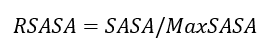
其中,SASA是溶剂可及表面积,MaxSASA是氨基酸最大溶剂可及表面积,单位均为Å。
为了测量氨基酸侧链的相对溶剂可及表面积,通常采用从Gly-X-Gly三肽中获得的MaxSASA值,其中X为需要计算的氨基酸残基。几种MaxSASA量表如下所示。
| Residue | Tien et al. 2013 (theor.)[1] | Tien et al. 2013 (emp.)[1] | Miller et al. 1987[2] | Rose et al. 1985[3] |
|---|---|---|---|---|
| Alanine | 129.0 | 121.0 | 113.0 | 118.1 |
| Arginine | 274.0 | 265.0 | 241.0 | 256.0 |
| Asparagine | 195.0 | 187.0 | 158.0 | 165.5 |
| Aspartate | 193.0 | 187.0 | 151.0 | 158.7 |
| Cysteine | 167.0 | 148.0 | 140.0 | 146.1 |
| Glutamate | 223.0 | 214.0 | 183.0 | 186.2 |
| Glutamine | 225.0 | 214.0 | 189.0 | 193.2 |
| Glycine | 104.0 | 97.0 | 85.0 | 88.1 |
| Histidine | 224.0 | 216.0 | 194.0 | 202.5 |
| Isoleucine | 197.0 | 195.0 | 182.0 | 181.0 |
| Leucine | 201.0 | 191.0 | 180.0 | 193.1 |
| Lysine | 236.0 | 230.0 | 211.0 | 225.8 |
| Methionine | 224.0 | 203.0 | 204.0 | 203.4 |
| Phenylalanine | 240.0 | 228.0 | 218.0 | 222.8 |
| Proline | 159.0 | 154.0 | 143.0 | 146.8 |
| Serine | 155.0 | 143.0 | 122.0 | 129.8 |
| Threonine | 172.0 | 163.0 | 146.0 | 152.5 |
| Tryptophan | 285.0 | 264.0 | 259.0 | 266.3 |
| Tyrosine | 263.0 | 255.0 | 229.0 | 236.8 |
| Valine | 174.0 | 165.0 | 160.0 | 164.5 |
通常有以下标准:
rASA >0.5(50%):残基被认为是暴露于溶液的(solvent-exposed)
rASA < 0.2(20%):残基被认为是埋藏在蛋白质内部的(buried)
0.2 ≤ rASA ≤ 0.5:残基处于部分暴露状态。
具体阈值的选择可能取决于研究的目的。例如,某些分析可能使用更严格或宽松的标准来划分。
蛋白的结构文件,PDB格式。
计算出来的各种溶剂可及表面积值,可根据需求选择需要的类型:
| 字段名称 | 说明 |
|---|---|
| ResidueType | 残基类型 |
| Chain ID | 链名称 |
| Residue Number | 残基编号 |
| total | Total SASA of residue |
| polar | Polar SASA(极性) |
| apolar | Apolar SASA(非极性) |
| mainChain | Main chain SASA |
| sideChain | Side chain SASA |
| relativeTotal* | Relative total SASA |
| relativePolar | Relative polar SASA |
| relativeApolar | Relative Apolar SASA |
| relativeMainChain | Relative main chain SASA |
| relativeSideChain* | Relative side chain SASA |
| bfactor | 温度因子 |
*常用的比如:
通常有以下标准:
rASA >0.5(50%):残基被认为是暴露于溶液的(solvent-exposed)
rASA < 0.2(20%):残基被认为是埋藏在蛋白质内部的(buried)
0.2 ≤ rASA ≤ 0.5:残基处于部分暴露状态。
具体阈值的选择可能取决于研究的目的。例如,某些分析可能使用更严格或宽松的标准来划分。
https://en.wikipedia.org/wiki/Relative_accessible_surface_area
Tien MZ, Meyer AG, Sydykova DK, Spielman SJ, Wilke CO. Maximum allowed solvent accessibilites of residues in proteins. PLoS One. 2013 Nov 21;8(11):e80635.
Miller S, Lesk AM, Janin J, Chothia C. The accessible surface area and stability of oligomeric proteins. Nature. 1987 Aug 27-Sep 2;328(6133):834-6.
Rose GD, Geselowitz AR, Lesser GJ, Lee RH, Zehfus MH. Hydrophobicity of amino acid residues in globular proteins. Science. 1985 Aug 30;229(4716):834-8.
https://freesasa.github.io/doxygen/Geometry.html
Based on protein structure (PDB file), calculates the solvent exposure of each residue (solvent accessible surface area, SASA). The relative solvent accessible surface area (RSASA) of protein amino acid residues measures the exposure of residues in the solvent. The calculation formula is as follows:
Here, SASA is the solvent accessible surface area, and MaxSASA is the maximum solvent accessible surface area of the amino acid, both in Å units. To measure the relative solvent accessible surface area of amino acid side chains, the MaxSASA value obtained from the Gly-X-Gly tripeptide is typically used, where X represents the amino acid residue being calculated. Several MaxSASA scales are shown below.
| Residue | Tien et al. 2013 (theor.)[1] | Tien et al. 2013 (emp.)[1] | Miller et al. 1987[2] | Rose et al. 1985[3] |
|---|---|---|---|---|
| Alanine | 129.0 | 121.0 | 113.0 | 118.1 |
| Arginine | 274.0 | 265.0 | 241.0 | 256.0 |
| Asparagine | 195.0 | 187.0 | 158.0 | 165.5 |
| Aspartate | 193.0 | 187.0 | 151.0 | 158.7 |
| Cysteine | 167.0 | 148.0 | 140.0 | 146.1 |
| Glutamate | 223.0 | 214.0 | 183.0 | 186.2 |
| Glutamine | 225.0 | 214.0 | 189.0 | 193.2 |
| Glycine | 104.0 | 97.0 | 85.0 | 88.1 |
| Histidine | 224.0 | 216.0 | 194.0 | 202.5 |
| Isoleucine | 197.0 | 195.0 | 182.0 | 181.0 |
| Leucine | 201.0 | 191.0 | 180.0 | 193.1 |
| Lysine | 236.0 | 230.0 | 211.0 | 225.8 |
| Methionine | 224.0 | 203.0 | 204.0 | 203.4 |
| Phenylalanine | 240.0 | 228.0 | 218.0 | 222.8 |
| Proline | 159.0 | 154.0 | 143.0 | 146.8 |
| Serine | 155.0 | 143.0 | 122.0 | 129.8 |
| Threonine | 172.0 | 163.0 | 146.0 | 152.5 |
| Tryptophan | 285.0 | 264.0 | 259.0 | 266.3 |
| Tyrosine | 263.0 | 255.0 | 229.0 | 236.8 |
| Valine | 174.0 | 165.0 | 160.0 | 164.5 |
Protein structure file in PDB format.
Calculated solvent accessible surface area values for various residue types can be selected as needed:
| Field Name | Description |
|---|---|
| ResidueType | Residue type |
| Chain ID | Chain name |
| Residue Number | Residue number |
| total | Total SASA of residue |
| polar | Polar SASA |
| apolar | Apolar SASA |
| mainChain | Main chain SASA |
| sideChain | Side chain SASA |
| relativeTotal* | Relative total SASA |
| relativePolar | Relative polar SASA |
| relativeApolar | Relative Apolar SASA |
| relativeMainChain | Relative main chain SASA |
| relativeSideChain* | Relative side chain SASA |
| bfactor | Temperature factor |
*Commonly used include:
Typically, the following criteria are used:
rASA > 0.5 (50%): Residues are considered solvent-exposed.
rASA < 0.2 (20%): Residues are considered buried within the protein.
0.2 ≤ rASA ≤ 0.5: Residues are in a partially exposed state.
The choice of specific thresholds may depend on the purpose of the study. For example, some analyses may use stricter or more lenient criteria for classification.
Relative accessible surface area - Wikipedia
Tien MZ, Meyer AG, Sydykova DK, Spielman SJ, Wilke CO. Maximum allowed solvent accessibilities of residues in proteins. PLoS One. 2013 Nov 21;8(11):e80635.
Miller S, Lesk AM, Janin J, Chothia C. The accessible surface area and stability of oligomeric proteins. Nature. 1987 Aug 27-Sep 2;328(6133):834-6.
Rose GD, Geselowitz AR, Lesser GJ, Lee RH, Zehfus MH. Hydrophobicity of amino acid residues in globular proteins. Science. 1985 Aug 30;229(4716):834-8.
Geometry - FreeSASA Documentation
基于MAFFT的多序列比对工具,支持蛋白和核酸序列的比对。
蛋白或者核酸的序列文件,FASTA格式
输出结果为多序列比对后的结果文件:alignment.fasta
Katoh K, Kuma K, Toh H, Miyata T. MAFFT version 5: improvement in accuracy of multiple sequence alignment. Nucleic Acids Res. 2005 Jan 20;33(2):511-8.
https://mafft.cbrc.jp/alignment/software/manual/manual.html
MAFFT-based tool for multiple sequence alignment, supports alignment of both protein and nucleic acid sequences.
Sequence file containing protein or nucleic acid sequences in FASTA format.
The output result is the aligned sequences saved in the file: alignment.fasta.
Katoh K, Kuma K, Toh H, Miyata T. MAFFT version 5: improvement in accuracy of multiple sequence alignment. Nucleic Acids Res. 2005 Jan 20;33(2):511-8.
MAFFT Manual
Antibody Sequence Prediction(IgLM)模块是抗体序列生成与优化,该方法从Observed Antibody Space (OAS) 收集抗体序列。OAS数据库包含六个物种的天然抗体序列:人类、小鼠、大鼠、兔子、恒河猴和骆驼。为了研究模型能力的影响,训练了两个版本的模型: IgLM和IgLM-S,分别有13M和1.4M的训练参数。两个IgLM模型都在558万非冗余序列上训练,这些序列基于95%相似性聚类。在训练过程中,随机屏蔽了抗体序列中10到20个残基,以便在推理过程中实现任意跨度的多样化。此外,还对序列中的链型(重链或轻链)和原产物种进行了限定,提供这样的背景能够控制物种特异性抗体序列的产生。该方法被证明可以从各种物种中产生全长的重链和轻链序列,以及具有改进可开发性的填充CDR环库。该方法是一个强大的抗体设计工具,可应用于各种抗体序列设计场景。
抗体序列,仅支持1条序列,FASTA格式。
设定为抗体重链或轻链,值为"H" 或 “L”。
指定序列中进行改造优化的氨基酸起始值,整数值,从1开始。需要说明的是,并不是说从优化起始值-终止值的氨基酸就会完全一对一的进行修改,模型里是指定开始到结束的残基作为1个MASK TOKEN提供给模型进行生成,具体生成多少个残基,是看模型学习的情况。
指定序列中进行改造优化的氨基酸终止值,整数值。需要说明的是,并不是说从优化起始值-终止值的氨基酸就会完全一对一的进行修改,模型里是指定开始到结束的残基作为1个MASK TOKEN提供给模型进行生成,具体生成多少个残基,是看模型学习的情况。
设定物种信息,默认是人源。
设定设计的序列数量,默认100。
输出结果文件为generated_seqs.fasta,包含生产的序列信息,fasta格式。
The Antibody Sequence Prediction (IgLM) module is designed for antibody sequence generation and optimization. This method collects antibody sequences from the Observed Antibody Space (OAS) database, which includes natural antibody sequences from six species: human, mouse, rat, rabbit, cynomolgus monkey, and camel. To study the impact of model capacity, two versions of the model were trained: IgLM and IgLM-S, with 13M and 1.4M training parameters, respectively. Both IgLM models were trained on 5.58 million non-redundant sequences clustered at 95% similarity. During training, 10 to 20 residues in the antibody sequences were randomly masked to achieve diversity across arbitrary spans during inference. Additionally, constraints were placed on the chain type (heavy or light chain) and original species in the sequences to control the generation of species-specific antibody sequences. This method has been shown to generate full-length heavy and light chain sequences from various species, along with a diversified CDR loop library for improved developability. It serves as a powerful antibody design tool applicable to various antibody design scenarios.
Antibody sequence in FASTA format, supporting only one sequence.
Specify the antibody chain type as heavy (“H”) or light (“L”).
Specify the starting amino acid index for optimization in the sequence, an integer value starting from 1. Note that the optimization does not necessarily modify each amino acid from the start to end index one-to-one. The model treats the specified residues from the start to end as one MASK TOKEN for generating sequences, and the actual number of residues generated depends on the model’s learning.
Specify the ending amino acid index for optimization in the sequence, an integer value. Similarly, the optimization does not necessarily modify each amino acid from the start to end index one-to-one.
Set the species information, default is human.
Set the number of sequences to be designed, default is 100.
The output result file is named generated_seqs.fasta, containing the information of the generated sequences in FASTA format.
PTM Hotspot by Structure模块通过快速的蒙特卡罗模拟采样,获得蛋白的多样性构象,通过分析多构象的溶剂暴露情况和结构波动情况来预测天冬氨酸(ASP)的异构化的概率。
蛋白的结构文件,格式支持 .pdb 或 .cif。支持多个复合物结构打包进行批量预测,格式支持 .tar、.tar.gz 、 .zip等,最大支持10个结构。
输出结果文件为result.csv,包含信息如下:
| 字段名称 | 说明 |
|---|---|
| Chain | 蛋白链名称 |
| Residue Index | 氨基酸索引(PDB文件中) |
| Pred_Score | 预测得到的ASP残基异构化评分,分数值在0-1之间,越大表示异构化的可能性越高 |
| Labile | 最终判别异构化的值,1表示预测发生异构化,0表示预测无异构化 |
| sasa_asp | ASP 残基侧链的 SASA(Solvent Accessible Surface Area,溶剂可及表面积)。数值越大表示该位点越暴露于溶剂,更容易发生化学修饰。单位通常为 Ų。 |
| rmsf | 残基结构波动反映蒙特卡罗采样过程中该残基的构象柔性。数值越大表示局部结构越灵活。单位通常为 Å。 |
| sasa_n_1 | 前一个残基主链氮原子的溶剂暴露 |
The PTM Hotspot by Structure module uses rapid Monte Carlo simulation sampling to obtain diverse protein conformations. By analyzing the solvent exposure and structural fluctuations of multiple conformations, it predicts the probability of aspartic acid (ASP) isomerization.
Protein structure file. Supported formats: .pdb or .cif. Batch prediction is supported by packaging multiple complex structures into archives. Supported archive formats: .tar, .tar.gz, .zip, etc. Maximum 10 structures.
The output result file is named result.csv, containing the following information:
| Field Name | Description |
|---|---|
| Chain | Name of the protein chain |
| Residue Index | Amino acid index (in the PDB file) |
| Pred_Score | Predicted score for ASP residue isomerization, with values ranging from 0 to 1; higher values indicate a higher likelihood of isomerization |
| Labile | Final determination of isomerization; 1 indicates predicted isomerization, 0 indicates predicted non-isomerization |
| sasa_asp | SASA (Solvent Accessible Surface Area) of the ASP residue side chain. Higher values indicate greater solvent exposure, making the site more susceptible to chemical modification. Unit: typically Ų. |
| rmsf | Residue structural fluctuation reflects the conformational flexibility of the residue during Monte Carlo sampling. Higher values indicate greater local structural flexibility. Unit: typically Å. |
| sasa_n_1 | Solvent exposure of the backbone nitrogen atom of the preceding residue |

Protein Isoelectric Point(pI),即分子不带净电荷的pH值,是影响分子理化性质甚至功能的关键参数。该模块使用多种不同的算法,基于序列计算分子的pI数值,并可以对多条链的结果进行合并计算。
基于唯信团队使用部分内部抗体实测pI数据的对比,Sillero算法的精度相对更高,推荐采用。
唯信测试用的抗体分子和对应的实测pI数值区间和均值如下图所示。
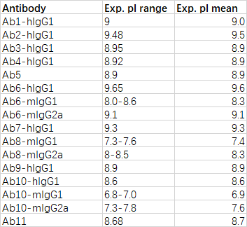
用不同算法计算的pI数值与实测均值的差值及相关性如下图所示。
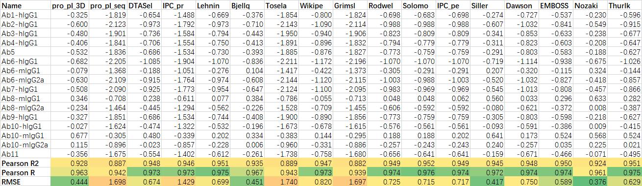
基于R和RMSE等指标,Sillero的相关性略优于其他算法。
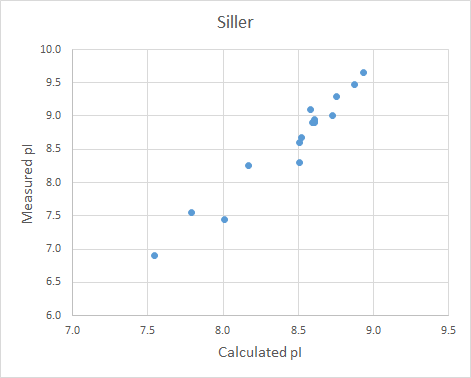
蛋白的序列文件,FASTA格式。
使用所选模型预测pI的输出文件,默认名称result.csv。
绘制二维散点图,默认False。
二维散点图(分子量与等电点)表示为热图,默认名称result.png。
根据链名,将来自同一序列的多条链的pI值进行合并计算。
例如:mol1.chain1与mol1.chain2将被合并为mol1分子的结果。同名的链也会被视为同一个分子。
仅当merge_chain=True时可用。默认值:merged.csv。
并行任务数,默认为1。
输出结果包括:
| 输出文件名称 | 说明 |
|---|---|
| result.png | 当Plot=True时输出二维散点图(分子量与等电点),热图形式 |
| result.csv | 使用所选模型预测pI的输出文件 |
| merged.csv | 多条链的pI合并输出文件 |
其中result.csv包括信息如下:
| 字段名称 | 说明 |
|---|---|
| Protein ID | 蛋白序列名称 |
| Molecular weight (Da) | 蛋白分子量 |
| pI | 蛋白等电点 |
Kozlowski LP. IPC - Isoelectric Point Calculator. Biol Direct. 2016 Oct 21;11(1):55.
Protein Isoelectric Point (pI), the pH at which a molecule carries no net charge, is a key parameter that influences the physical and functional properties of a molecule. This module uses various algorithms to calculate the pI value of a molecule based on its sequence and can merge results for multiple chains.
Based on a comparison of experimentally measured pI data from a subset of internal antibodies by the WeiXin team, the Sillero algorithm demonstrates relatively higher accuracy and is recommended for use.
The figure below shows the antibody molecules used in the WeiXin tests along with the corresponding ranges and averages of experimentally measured pI values.
The figure below illustrates the differences and correlations between the pI values calculated using different algorithms and the experimentally measured averages.
Based on metrics such as R and RMSE, the Sillero algorithm shows slightly better correlation compared to other algorithms.
File containing the protein sequence in FASTA format.
Output file for predicted pI values using the selected model, default name is result.csv.
Whether to plot a two-dimensional scatter plot, default is False.
Graphical representation of the two-dimensional scatter plot (molecular weight vs. isoelectric point), default name is result.png.
Merge pI values of multiple chains from the same sequence based on chain names.
For example: mol1.chain1 and mol1.chain2 will be merged into the result for the molecule mol1. Chains with the same name are considered as part of the same molecule.
Available only when merge_chain=True, default value is merged.csv.
Number of parallel tasks, default is 1.
The output includes:
| Output File Name | Description |
|---|---|
| result.png | Output of the two-dimensional scatter plot (molecular weight vs. isoelectric point) if Plot=True, in heatmap format |
| result.csv | Output file for predicted pI values using the selected model |
| merged.csv | Merged output file for pI values of multiple chains |
The result.csv file includes the following information:
| Field Name | Description |
|---|---|
| Protein ID | Protein sequence name |
| Molecular weight (Da) | Protein molecular weight |
| pI | Protein isoelectric point |
Kozlowski LP. IPC - Isoelectric Point Calculator. Biol Direct. 2016 Oct 21;11(1):55.
AlphaFold2是目前业界优秀的蛋白质结构预测方法。由Deepmind 团队开发,在2020年的蛋白质结构预测大赛CASP14中, AlphaFold 2 得到了接近90分的成绩,排名第一,大幅度领先第二名,对大部分蛋白质结构的预测与真实结构只差一个原子的宽度,达到了人类利用冷冻电镜等复杂仪器观察预测的水平,这是蛋白质结构预测史无前例的巨大进步。后续更新版本支持复合物结构预测,包括蛋白-多肽复合物的预测。
当前版本:v2.3.2, 是截止于2023年10月的最新版本。
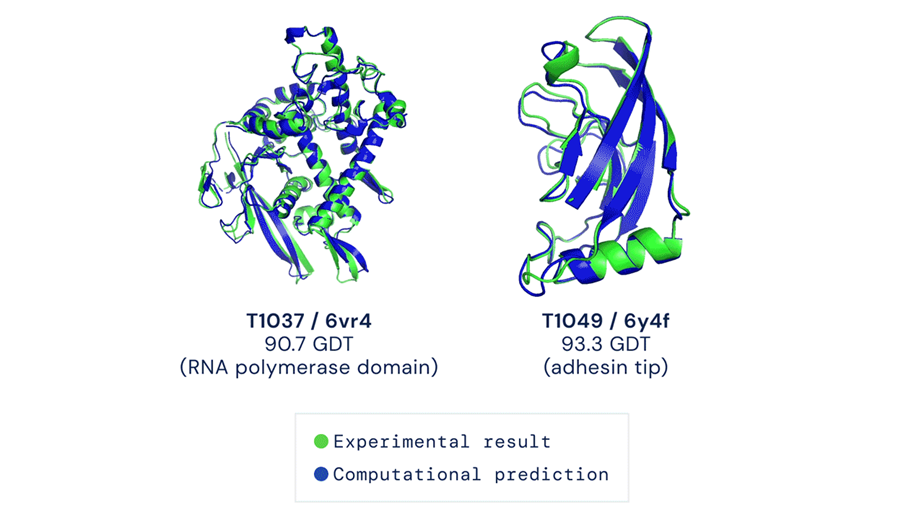
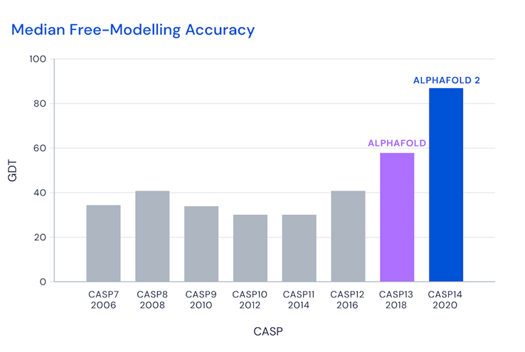
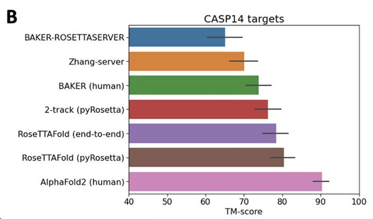
上图:蛋白单体预测精度
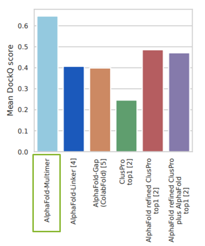
上图:蛋白复合物预测精度
输入序列文件,fasta格式
预测任务类型,monomer 或者 multimer
monomer:单体蛋白,单条链
multimer:复合物,多条链,最大可以6条链,超过6条系统不处理
优化结构模式
all:优化所有的结构
best:只优化打分最高的结构,这个模式只输出一个结构
none:不做优化
多序列比对使用的数据库
full_dbs:全库,更耗时,但相比reduced_db更精确
reduced_dbs:精简库,速度更快,但是牺牲准确性
输出结果包括:
| 输出文件名称 | 说明 |
|---|---|
| ranking_debug.csv | 预测模型可信度评估文件,其中包含用于执行模型排名的pLDDT, ipTM, pTM值,以及到原始模型名称的映射。 |
| ranked_*.pdb | 预测最终蛋白结构文件。默认提供1个打分最高的优化后的结构 |
| PAE_0.csv | 当预测为复合物结构时,生成最优模型的Predicted aligned error(PAE)热图CSV数据。 |
| PAE_Heatmap_0.png | 当预测为复合物结构时,生成最优模型的Predicted aligned error(PAE)热图。 |
| PAE.tar.gz | 当预测为复合物结构时,生成所有模型的Predicted aligned error(PAE)热图。 |
其中评估结构预测可信度指标分为pLDDT和ipTM:
pLDDT > 90:Very high
90 > pLDDT > 70:Confident
70 > pLDDT > 50:Low
pLDDT < 50:Very low
model confidence = 0.8 · ipTM + 0.2 · pTM,值范围是0-1,该值越大说明预测的复合物结构越可靠。
ipTM >= 0.80:High quality
0.6 <= ipTM < 0.80:Acceptable quality
0.00 <= ipTM < 0.6:Incorrect
对结构准确性分析应该综合考虑所有指标,包括pTM、ipTM、pLDDT 和 PAE。
AlphaFold2 is currently the best protein structure prediction method in the industry. Developed by the DeepMind team, in the 2020 CASP14 protein structure prediction competition, AlphaFold 2 achieved a score close to 90, ranking first and significantly outperforming the second-place competitor. It predicted the structures of most proteins within the width of a single atom from the ground truth, reaching a level comparable to human observation using complex instruments like cryo-electron microscopy. This represents an unprecedented advancement in protein structure prediction. Subsequent updates support the prediction of complex structures, including protein-peptide complexes.
Current Version: v2.3.2, the latest version as of October 2023.
Above: Protein monomer prediction accuracy
Above: Protein complex prediction accuracy
Input sequence file in FASTA format.
Prediction task type, either monomer or multimer.
monomer: Single protein, single chain.
multimer: Complex, multiple chains, with a maximum of 6 chains. Systems with more than 6 chains are not processed.
Structure optimization mode.
all: Optimize all structures.
best: Optimize only the highest-scoring structure; this mode outputs only one structure.
none: No optimization.
Database used for multiple sequence alignment.
full_dbs: Full database, more time-consuming but more accurate compared to reduced_db.
reduced_dbs: Reduced database, faster but sacrifices accuracy.
The output includes:
| Output File Name | Description |
|---|---|
| ranking_debug.csv | Confidence evaluation file of the prediction model, containing pLDDT, ipTM, pTM values used for model ranking and mapping to the original model names. |
| ranked_*.pdb | Final predicted protein structure files. By default, the optimized highest-scoring structure is provided. |
| PAE_0.csv | For complex structure predictions, generates a Predicted Aligned Error (PAE) heatmap CSV data for the best model. |
| PAE_Heatmap_0.png | For complex structure predictions, generates a Predicted Aligned Error (PAE) heatmap for the best model. |
| PAE.tar.gz | For complex structure predictions, generates PAE heatmaps for all models. |
The confidence metrics for structure prediction include pLDDT and DockQ:
pLDDT > 90: Very high
90 > pLDDT > 70: Confident
70 > pLDDT > 50: Low
pLDDT < 50: Very low
model confidence = 0.8 · ipTM + 0.2 · pTM. The value ranges from 0 to 1, with higher values indicating a more reliable predicted complex structure.
ipTM >= 0.80: High quality
0.6 <= ipTM < 0.80: Acceptable quality
0.00 <= ipTM < 0.6: Incorrect
粘度是影响抗体药物开发的重要因素,临床上抗体往往需要静脉内或皮下给药,需要高浓度的抗体溶液(>100mg/mL)才能以小剂量注射获得与治疗相关的剂量,但是高浓度的抗体往往表现出高粘度,这对抗体药物的开发,制造和给药提出了挑战。研究发现,抗体序列是决定抗体粘度的关键因素,文献报道抗体粘度与Fv区域的电荷、VH和VL区域电荷的不对称性FvCSP和Fv区域的疏水指数HI存在相关性,基于抗体序列预测抗体粘度是一个有效方法。
本模块集成了两种粘度预测方法:Sharma 与 DeepViscosity
Sharma 粘度计算方法如下所示:
η,cP(180 mg/mL,25°C)=10^[0.15+1.26(0.60)∗ϕ−0.043(0.047)∗q−0.020(0.015)∗qsym
其中,ϕ代表Fv区域的疏水指数HI,q代表Fv电荷,qsym代表VH和VL区域电荷的不对称性FvCSP。
DeepViscosity模型是一个集成了102个人工神经网络模型的集成学习系统。该模型利用从抗体序列(特别是Fv区)提取的30种特征,对单抗进行粘度分类。分类标准基于150mg/mL浓度下的粘度值,区分低粘度(≤20 cP)和高粘度(>20 cP)的抗体。使用了包含 229 种不同单抗及其在150mg/mL浓度下实验测定粘度值的大型数据集来训练 DeepViscosity。该数据集是目前该领域公开报道的最大的同类数据集,为模型的稳健性提供了坚实基础。 在两个独立的测试集上进行的评估结果显示,DeepViscosity 表现出色。该模型在这两个测试集上分别达到了 87.5% 和 89.5% 的粘度分类准确率,其性能显著超越了以往依赖实验数据或复杂计算模拟的预测模型。
抗体的序列文件,FASTA格式,支持批量抗体,不支持纳米抗体序列。序列按要求使用分子名.链名的形式进行命名,示例如下:
> 抗体A.H
重链序列XXXXXX
> 抗体A.L
轻链序列XXXXXX
> 抗体B.L
轻链序列XXXXXX
> 抗体B.H
重链序列XXXXXX
输出结果文件,默认为vis_pred_res_SM.csv
抗体的序列文件,FASTA格式(格式要求同Sharma模式)
输出结果文件,默认为vis_pred_res_DV.csv
Sharma算法输出vis_pred_res_SM.csv文件,包含信息如下:
| 字段名称 | 说明 |
|---|---|
| Sequence ID | 抗体序列名称 |
| Fv Heavy Chain Charge | 重链电荷 |
| Fv Light Chain Charge | 轻链电荷 |
| Fv Charge Symmetry Parameter | 电荷对称性指标 |
| Fv Hydrophobicity Index | 疏水性指数 |
| Viscosity | 抗体粘度 |
DeepViscosity算法输出vis_pred_res_DV.csv文件,包含信息如下:
| 字段名称 | 说明 |
|---|---|
| Sequence ID | 抗体序列名称 |
| Viscosity Type | 预测的抗体粘度类别,0表示低粘度(≤20 cP),1表示高粘度(>20 cP) |
| Probability | 预测的概率值,数值在0-1之间,大于0.5时Viscosity Type为1,反之为0 |
Viscosity is an important factor affecting the development of antibody drugs. Clinically, antibodies often need to be administered intravenously or subcutaneously, requiring a high concentration of antibody solution (>100mg/mL) to obtain a therapeutic dose at a small dose. However, high concentrations of antibodies often exhibit high viscosity, which poses a challenge to the development, manufacture and administration of antibody drugs. It has been found that antibody sequence is the key factor to determine antibody viscosity. It has been reported that antibody viscosity is correlated with charge in Fv region, charge asymmetry in VH and VL region, FvCSP, and hydrophobic index HI in Fv region. It is an effective method to predict antibody viscosity based on antibody sequence.
This module integrates two viscosity prediction methods: Sharma and DeepViscosity.
Sharma method:
η,cP(180 mg/mL,25°C)=10^[0.15+1.26(0.60)∗ϕ−0.043(0.047)∗q−0.020(0.015)∗qsym
Among them, ϕ represents the hydrophobic index (HI) of the Fv region, q represents the charge of the Fv region, and qsym represents the asymmetry of the charge in the VH and VL regions (FvCSP).
The DeepViscosity model is an ensemble learning system that incorporates 102 artificial neural network models. It uses 30 features extracted from antibody sequences (especially the Fv region) to classify monoclonal antibodies based on their viscosity. The classification criterion is based on the viscosity value at a concentration of 150 mg/mL, distinguishing between low viscosity (≤20 cP) and high viscosity (>20 cP) antibodies. The model was trained using a large dataset containing 229 different monoclonal antibodies and their experimentally measured viscosity values at a concentration of 150 mg/mL. This dataset is the largest of its kind reported in the field to date, providing a solid foundation for the robustness of the model. Evaluation results on two independent test sets show that DeepViscosity performs remarkably well. The model achieved viscosity classification accuracies of 87.5% and 89.5% on the two test sets, respectively, significantly outperforming previous prediction models that relied on experimental data or complex computational simulations.
Antibody sequence file in FASTA format. Supports multiple antibodies, but does not support nanobody sequences. The sequence is named in the form of molecule name.chain name as required. as shown in the example below.:
> antibodyA.H
XXXXXX(Heavy chain)
> antibodyA.L
XXXXXX(Light chain)
> antibodyB.L
XXXXXX(Light chain)
> antibodyB.H
XXXXXX(Heavy chain)
The output result file, default name is vis_pred_res_SM.csv
The sequence file of the antibody, in FASTA format (the format requirements are the same as those in Sharma mode)
The output result file, default name is vis_pred_res_DV.csv
A result.csv file contains the following information:
| Field Name | Description |
|---|---|
| Sequence ID | Antibody sequence name |
| Fv Heavy Chain Charge | Fv heavy chain charge |
| Fv Light Chain Charge | Fv light chain charge |
| Fv Charge Symmetry Parameter | Fv charge symmetry index |
| Fv Hydrophobicity Index | Fv hydrophobicity index |
| Viscosity | Antibody viscosity |
The output file of the DeepViscosity algorithm is named vis_pred_res_DV.csv, which contains the following information:
| Field Name | Description |
|---|---|
| Sequence ID | Name of the antibody sequence |
| Viscosity Type | Predicted viscosity category of the antibody. 0 indicates low viscosity (≤20 cP), and 1 indicates high viscosity (>20 cP) |
| Probability | The predicted probability value ranges between 0 and 1. When it is greater than 0.5, the Viscosity Type is 1; otherwise, it is 0. |
Molecular Docking (DiffDock)是一种扩散生成模型,主要用于小分子和蛋白对接。DiffDock在PDBBind上获得了38%的top-1成功率(RMSD<2A),大大超过了以前传统对接(23%)和深度学习(20%)方法的最先进水平。此外,以前的方法无法对接计算上的折叠结构(最大精度为10.4%),而DiffDock保持了明显更高的精度(21.7%)。最后,DiffDock具有快速的推理时间,并提供具有高选择性精度的置信度估计值。
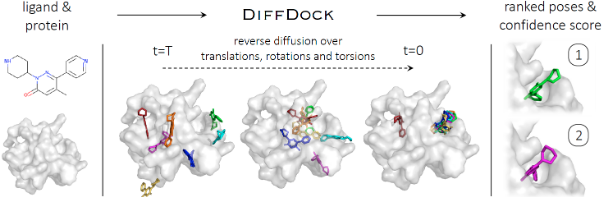
蛋白的结构文件,PDB格式。最多支持1022个氨基酸。
小分子结构文件,SDF格式
每个配体与受体对接时得到的构象数,默认为10。
输出结果包括:
| 输出文件名称 | 说明 |
|---|---|
| Scores.csv | 所有配体(≤2000)与受体的打分文件。 |
| output_ligand.sdf | 对接后所有配体SDF文件。 |
| output_complex_topn.tar.gz | TopN小分子中每个配体与受体打分最高的复合物构象PDB文件压缩包。 |
| display_complex.pdb | 展示配体与受体的复合物构象文件。 |
其中Scores.csv包含信息如下:
| 字段名称 | 说明 |
|---|---|
| Ligand ID | 配体编号ID |
| Confidence | 对接置信度打分,虽然解读和比较不同复合物或不同蛋白质构象的置信度分数可能会很困难,可以通过以下标准粗略比较(c是最佳构象的置信度分数):c > 0高置信度;-1.5 < c < 0中等置信度;c < -1.5低置信度 |
| Complex File Name | 复合物名称 |
Molecular Docking (DiffDock) is a diffusion-based model primarily used for the docking of small molecules with proteins. DiffDock has achieved a top-1 success rate of 38% (RMSD < 2A) on PDBBind, significantly surpassing the state-of-the-art levels of previous traditional docking methods (23%) and deep learning methods (20%). Furthermore, previous methods were unable to dock computationally folded structures (maximum accuracy of 10.4%), while DiffDock maintains significantly higher accuracy (21.7%). Finally, DiffDock features fast inference times and provides confidence estimates with high selectivity accuracy.
Structure file of the protein in PDB format. Supports up to 1022 amino acids.
Structure file of the small molecule in SDF format.
The number of conformations obtained for each ligand docked with the receptor, default is 10.
The output includes:
| Output File Name | Description |
|---|---|
| Scores.csv | Scoring file for all ligands (≤2000) with the receptor. |
| output_ligand.sdf | SDF file containing all ligands after docking. |
| output_complex_topn.tar.gz | Compressed file containing the PDB files of the top scoring complex conformations for each ligand among the TopN small molecules. |
| display_complex.pdb | File displaying the complex conformation of the ligand and receptor. |
The Scores.csv contains the following information:
| Field Name | Description |
|---|---|
| Ligand ID | Ligand identification ID. |
| Confidence | Docking confidence score. Although interpreting and comparing confidence scores of different complexes or different protein conformations can be challenging, a rough comparison can be made using the following criteria (c is the confidence score of the top pose): c > 0 indicates high confidence; -1.5 < c < 0 indicates moderate confidence; c < -1.5 indicates low confidence. |
| Complex File Name | Name of the complex. |
Synthetic Accessibility Score是一个化合物合成可行性评估指标,反映了化合物是否容易合成。其将小分子合成难易程度用1到10区间数值进行评价,越靠近1表明越容易合成,越靠近10表明合成越困难。SA Score基于片段贡献和复杂度惩罚从而评估化合物合成的难易程度,其中片段贡献值根据PubChem数据库中上百万分子计算共性进行计算,复杂度则考虑分子中非标准结构特征的占比,例如大环、非标准环的合并、立体异构和分子量大小等方面。SA Score方法已被验证,通过将40个化合物分别采用SA Score和经验丰富的药物化学家评估其合成难易程度,并且比较得到二者评分的相关性R2高达0.89,表明其在识别可合成难易程度上的可靠性较高。SA Score已成为一种普遍使用的指标,可用于预测新化合物的合成可行性,加速化合物筛选和药物发现过程。

小分子结构文件,支持SDF和SMILES格式。
小分子结构,SMILES格式,支持多个小分子,一行一个SMILES,例如:
CSC1=C(c2ccc©s2)/C(=N/C©©C)C1
CC1=C(C=C(C=C1)NC(=O)C2=CC=C(C=C2)CN3CCN(CC3)C)NC4=NC=CC(=N4)C5=CN=CC=C5
输出结果文件为sa_score.csv,包含信息如下:
| 字段名称 | 说明 |
|---|---|
| smiles | 小分子smiles结构 |
| Name | 小分子名称 |
| sa_score | 化合物合成可行性评估指标数值 |
The Synthetic Accessibility Score is an indicator of the feasibility of synthesizing a compound, reflecting how easily a compound can be synthesized. It evaluates the difficulty of synthesizing small molecules on a scale of 1 to 10, with values closer to 1 indicating easier synthesis and values closer to 10 indicating more challenging synthesis. The SA Score assesses the ease of compound synthesis based on fragment contributions and complexity penalties. The fragment contribution values are calculated based on the commonality of millions of molecules in the PubChem database, while complexity considers the proportion of non-standard structural features in the molecule, such as macrocycles, fused non-standard rings, stereoisomers, molecular weight, and other aspects. The SA Score method has been validated by comparing the SA Scores with evaluations of synthesis difficulty by experienced medicinal chemists for 40 compounds. The high correlation coefficient (R2 = 0.89) between the two sets of scores demonstrates the reliability of the SA Score in identifying the feasibility of synthesis. The SA Score has become a widely used metric for predicting the synthetic feasibility of new compounds, accelerating compound screening and drug discovery processes.
Small molecule structure file in SDF or SMILES format.
SMILES format of small molecule structures, supports multiple small molecules with one SMILES string per line, for example:
CSC1=C(c2ccc©s2)/C(=N/C©©C)C1
CC1=C(C=C(C=C1)NC(=O)C2=CC=C(C=C2)CN3CCN(CC3)C)NC4=NC=CC(=N4)C5=CN=CC=C5
The output file is sa_score.csv, containing the following information:
| Field Name | Description |
|---|---|
| smiles | SMILES structure of the small molecule |
| Name | Name of the small molecule |
| sa_score | Synthetic Accessibility Score value for the compound |
Cleavage Site Prediction (DeepDigest) 模块基于深度学习,用于预测8种常用蛋白酶(trypsin, ArgC, chymotrypsin, GluC, LysC, AspN, LysN, and LysargiNase)的蛋白型裂解位点。它整合了卷积神经网络和长短时记忆网络,以实现高准确性和稳健性。与传统的机器学习算法(逻辑回归、随机森林和支持向量机)相比,对所有8种蛋白酶都有更准确的预测精度。
以下是八种常用蛋白酶的蛋白型裂解位点预测:
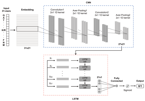
蛋白的序列文件,FASTA格式
输出对应8个蛋白酶的csv文件,每个csv文件包括信息如下:
| 字段名称 | 说明 |
|---|---|
| Protein id | 蛋白名称 |
| Peptide sequence | 蛋白的理论酶切肽段 |
| Digestibility of the N-terminal site | N端肽键的裂解概率预测值 |
| Digestibility of the C-terminal site | C端肽键的裂解概率预测值 |
| Digestibility of the missed site(s) | 理论酶切肽段所有漏切(非N/C端)位点的酶切概率预测值,这里漏切位点指的是:符合蛋白酶特异性、理论上应被切割,但实际实验中未被切割的肽键位点。以最常见的胰蛋白酶(trypsin)为例:酶切规则是K/R 后(非 P)切开,一条蛋白质序列为… A K G R T … 理论完全酶切是在K 后切、R 后切,若实际得到肽段 AKGRT,说明 K 后没切、R 后没切, 这两个位点就是 missed sites |
*注:概率值区间为0-1,越接近1表示发生概率越大。
Cleavage Site Prediction (DeepDigest) module is based on deep learning. Used to predict the protein-type cleavage sites of eight common proteases (trypsin, ArgC, chymotrypsin, GluC, LysC, AspN, LysN, and LysargiNase). It integrates convolutional neural network and short - and long-term memory network to achieve high accuracy and robustness. Compared with traditional machine learning algorithms (logistic regression, random forest and support vector machine), the prediction accuracy of all eight proteases was more accurate.
The following are protein-type cleavage site predictions for eight common proteases:

Protein sequence file in FASTA format
The output csv file is corresponding to the 8 proteases. Each csv file contains the following information:
| Field Name | Description |
|---|---|
| Protein id | The identity of the protein from which the peptide is digested. |
| Peptide sequence | The sequence of the theoretical digested peptide. |
| Digestibility of the N-terminal site | The predicted cleavage probability of the cleavage site on the N-terminal of the peptide. |
| Digestibility of the C-terminal site | The predicted cleavage probability of the cleavage site on the C-terminal of the peptide. |
| Digestibility of the missed site(s) | The predicted cleavage probabilities of the missed cleavage sites in the peptide. Here, “missed sites” (or “missed cleavage sites”) refer to peptide bond positions that meet the protease specificity and theoretically should be cleaved, but were not cleaved in actual experiments. Taking the most common trypsin as an example: the cleavage rule is to cut after K/R (not followed by P). For a protein sequence … A K G R T …, theoretical complete digestion would result in cleavage after K and after R. If the actual peptide obtained is AKGRT, this indicates no cleavage occurred after K or after R—these two positions are the missed sites. |
通过基于扩散概率模型,在蛋白质结构去噪任务上对RoseTTAFold结构预测网络进行微调,得到该蛋白质骨架生成模型,在无条件和拓扑约束的蛋白质单体设计、蛋白质结合物设计、对称低聚物设计、酶活性位点支架以及治疗性和金属结合蛋白设计的对称主题支架上取得了出色的性能。RFdiffusion能够从简单的分子规格中设计出多样的、复合的、功能性的蛋白质,也适用于环肽设计。
模块功能为多场景蛋白设计,如:Motif Scaffolding,Unconditional protein generation,Symmetric unconditional generation (cyclic, dihedral and tetrahedral symmetries),Symmetric motif scaffolding,Binder design,Design diversification (“partial diffusion”)
设计时的参考蛋白。
设计类型,支持2种类型:‘Motif_Scaffold’与’Binder’,分别说明如下:
‘Motif_Scaffold’ 表示基于参考蛋白的骨架结构(由后续参数定义),进行设计。
‘Binder’ 表示基于受体结构进行其Binder蛋白设计。
指定要设计的结构数量(目前最多支持 100 个)。
定义蛋白的设计策略,指定蛋白中的哪部分被随机设计、保留等。
如:该参数设置为 ‘5-15/A10-25/30-40/0 B1-100’ 时,
●’5-15’表示先设计长度为5到15之间(具体多长是随机的,如果要固定长度为10,可以设置为10-10)的motif
●‘/A10-25’表示紧接着从参考蛋白中取A链中编号为10至25的氨基酸,其N端连接到上一段’5-15’设计的motif的C端
●’/30-40’表示紧接着设计长度为30到40之间(具体多长是随机的)的motif,其N端连接到前面已经设计的motif的C端
●‘/0 ’表示链断开,前一条链结束,后续设计会是新的链,注意0后有一个空格!
●‘B1-100’表示从参考蛋白中取B链中编号为1至100的氨基酸,作为新的一条链
注意:
在binder模式下可以指定受体中的热点残基,格式为"链名称",“氨基酸残基”,如:‘A59,A83,A91’。
设计对称蛋白,参数值为C_N或D_N,其中C表示循环对称(Cyclic symmetry),D表示二面体对称(Dihedral symmetry),N表示单体的数量。如:C2表示设计包含2个单体的循环对称蛋白。
注意:在进行对称蛋白设计时,Contigs参数的设置要与之匹配,如:Symmetry为C2时,Contigs参数的设置应该符合两条链。
设计时的参考蛋白。
为后续参数(Receptor, Initial Binder, Hotspot)中定义的氨基酸残基的索引设置类别。
有两种选择:UID或者POS,UID表示PDB文件中自带的残基编号,该编号可能存在间断不连续,不从1开始等情况;POS表示位置编号或自然顺序编号,从1开始按顺序进行编号。
该参数的默认值为UID。
定义受体蛋白,从参考蛋白中选定哪部分作为受体蛋白,格式为“链名称+残基编号或范围”,多段残基用逗号分隔。例如:参数设置为A1-50,A70-100,A105,A108,B1-108时,表示:
选取参考蛋白的A链中残基编号为1至50、70至100、105与108的残基,以及B链位置编号1至108的残基作为受体。
注意:这里输入的残基编号应与参数Index Type中的编号类别一致。
定义Binder蛋白的长度,可以是确定的长度,或长度范围,例如:设置为20或20-50时,
20表示Binder蛋白的长度为20个残基;
20-50表示Binder蛋白的长度范围为20至50个残基,具体长度视最终设计结果为准。
指定要设计的结构数量(目前最多支持 100 个)。
指定结构中初始的Binder,从参考蛋白中选定哪部分是初始的Binder蛋白,模型会在不改变初始Binder的前提下,进一步延长Binder。例如:参数设置为B1-10时,表示:
指定参考蛋白中的B链残基编号为1至10的残基为初始Binder蛋白,模型会以此为基础进行延长设计。
指定受体中的热点残基作为binder蛋白的结合位置,格式为“链名称+残基编号或范围”,多段残基用逗号分隔,例如:A59-61,A83,A91,表示:
指定A链编号为59至61、83及91的残基为binder蛋白的结合位置。
设计时的参考蛋白。
为后续参数(Design Range)中定义的氨基酸残基的索引设置类别。
有两种选择:UID或者POS,UID表示PDB文件中自带的残基编号,该编号可能存在间断不连续,不从1开始等情况;POS表示位置编号或自然顺序编号,从1开始按顺序进行编号。
该参数的默认值为UID。
定义需要设计的蛋白骨架范围,从参考蛋白中选定哪部分进行设计,格式为“链名称+残基编号或范围”,多段残基用逗号分隔。例如:参数设置为A1-50,A70-100,A105,A108,B1-108时,表示:
选取参考蛋白的A链中残基编号为1至50、70至100、105与108的残基,以及B链编号1至108的残基进行骨架优化设计。
注意:这里输入的残基编号应与参数Index Type中的编号类别一致。
指定要设计的结构数量(目前最多支持 100 个)。
为参数Design Range中的每段残基,定义其设计的长度,多个长度用逗号分隔。如不设置该参数,表示按Design Range中的原始长度进行设计。
注意:长度的数量要与上述Range参数中残基段的数量一致,且顺序对应。长度可以有多种不同的取值:
N,表示该段残基区域设计时,长度不变。5-10,表示该段残基设计时,长度在5-10个残基的范围内变化,具体长度看最终设计结果。N,5-10,15表示定义了3个长度(对应的Design Range参数中的残基段应该也是3个),第1段残基设计时保持长度不变,第2段残基设计时的长度范围为5-10,第3段残基设计时的长度为15。其他设计模式,可选为Fix,表示固定上述定义的Design Range不变,对结构中的所有其他区域进行设计。
当其他设计模式设置为Fix时,会对其他区域进行设计,设计时会在其他区域的原长度基础上做长度变动,该参数即为长度变动的大小,默认为5,即在原长度的基础上减少或增加5个残基。
设计时的参考蛋白。
为后续参数(Receptor, Hotspot)中定义的氨基酸残基的索引设置类别。
有两种选择:UID或者POS,UID表示PDB文件中自带的残基编号,该编号可能存在间断不连续,不从1开始等情况;POS表示位置编号或自然顺序编号,从1开始按顺序进行编号。
该参数的默认值为UID。
定义受体蛋白,从参考蛋白中选定哪部分作为受体蛋白,格式为“链名称+残基编号或范围”,多段残基用逗号分隔。例如:参数设置为A1-50,A70-100,A105,A108,B1-108时,表示:
选取参考蛋白的A链中残基编号为1至50、70至100、105与108的残基,以及B链位置编号1至108的残基作为受体。
注意:
1.这里输入的残基编号应与参数Index Type中的编号类别一致。
2.同一链内的所有残基或范围必须按残基编号升序排列
定义环肽的长度,可以是确定的长度,或长度范围,例如:设置为10或12-18时,
10表示环肽蛋白的长度为10个残基;
12-16表示环肽的长度范围为12至16个残基,具体长度视最终设计结果为准。
指定受体中的热点残基作为binder蛋白的结合位置,格式为“链名称+残基编号或范围”,多段残基用逗号分隔,例如:A59-61,A83,A91,表示:
指定A链编号为59至61、83及91的残基为binder蛋白的结合位置。
设计得到的复合物结构pdb文件。
注意:
By fine-tuning the RoseTTAFold structure prediction network on protein structure denoising tasks through a diffusion probabilistic model, this protein backbone generation model was obtained, achieving excellent performance in unconditional and topology-constrained protein monomer design, protein complex design, symmetric oligomer design, enzyme active site scaffolding, and symmetric motif scaffolding for therapeutic and metal-binding protein design. RFdiffusion can design diverse, complex, and functional proteins from simple molecular specifications, and is also suitable for cyclic peptide design.
The module functions include multi-scenario protein design, such as: Motif Scaffolding, Unconditional protein generation, Symmetric unconditional generation (cyclic, dihedral and tetrahedral symmetries), Symmetric motif scaffolding, Binder design, and Design diversification (“partial diffusion”).
The reference protein for design.
Design type, supporting two types: ‘Motif_Scaffold’ and ‘Binder’, explained as follows:
Specifies the number of structures to design (currently supports up to 100).
Defines the protein design strategy, specifying which parts of the protein are randomly designed, retained, etc.
For example, if this parameter is set to ‘5-15/A10-25/30-40/0 B1-100’:
Note:
In binder mode, hotspot residues in the receptor can be specified, formatted as “chain name,” “amino acid residue,” e.g., ‘A59,A83,A91’.
Design symmetric proteins with parameter values C_N or D_N, where C indicates cyclic symmetry, D indicates dihedral symmetry, and N indicates the number of monomers. For example, C2 designs a cyclic symmetric protein with 2 monomers.
Note: When designing symmetric proteins, the Contigs parameter settings should match, e.g., if Symmetry is C2, the Contigs parameter should correspond to two chains.
The reference protein for design.
Sets the index type for amino acid residues defined in subsequent parameters (Receptor, Initial Binder, Hotspot). Two options are available: UID or POS. UID refers to the residue numbers provided in the PDB file, which may be discontinuous or not start from 1. POS refers to position numbering or natural sequential numbering starting from 1. The default value is UID.
Defines the receptor protein, selecting which parts from the reference protein serve as the receptor, formatted as “chain name + residue number or range,” separated by commas for multiple segments. For example, if the parameter is set to A1-50,A70-100,A105,A108,B1-108, it means:
Select residues numbered 1 to 50, 70 to 100, 105, and 108 from chain A, and residues numbered 1 to 108 from chain B of the reference protein as the receptor.
Note: The residue numbers entered here should match the index type specified in Index Type.
Defines the length of the Binder protein, which can be a specific length or a range. For example, setting it to 20 or 20-50 means:
20 specifies the Binder protein length as 20 residues;
20-50 specifies the Binder protein length range as 20 to 50 residues, with the exact length determined by the final design.
Specifies the number of structures to design (currently supports up to 100).
Specifies the initial Binder structure, selecting which parts from the reference protein are the initial Binder protein, with the model extending the Binder without changing the initial Binder. For example, if the parameter is set to B1-10, it means:
Specify residues numbered 1 to 10 from chain B of the reference protein as the initial Binder protein, and the model will extend the design based on this.
Specify hotspot residues in the receptor as binder protein binding sites, formatted as “chain name + residue number or range,” separated by commas for multiple segments. For example, A59-61,A83,A91 means:
Specify residues numbered 59 to 61, 83, and 91 in chain A as binder protein binding sites.
The reference protein for design.
Sets the index type for amino acid residues defined in subsequent parameters (Design Range). Two options are available: UID or POS. UID refers to the residue numbers provided in the PDB file, which may be discontinuous or not start from 1. POS refers to position numbering or natural sequential numbering starting from 1. The default value is UID.
Defines the protein backbone range to design, selecting which parts from the reference protein to optimize, formatted as “chain name + residue number or range,” separated by commas for multiple segments. For example, if the parameter is set to A1-50,A70-100,A105,A108,B1-108, it means:
Select residues numbered 1 to 50, 70 to 100, 105, and 108 from chain A, and residues numbered 1 to 108 from chain B of the reference protein for backbone optimization design.
Note: The residue numbers entered here should match the index type specified in Index Type.
Specifies the number of structures to design (currently supports up to 100).
Defines the design length for each segment in the Design Range parameter, with multiple lengths separated by commas. If this parameter is not set, the design length will follow the original length in the Design Range. Note: The number of lengths must match the number of residue segments in the Range parameter, and the order must correspond. Length can have various values:
N, indicating the segment length remains unchanged during design.5-10, indicating the segment design length varies between 5 and 10 residues, with the exact length determined by the final design.N,5-10,15 defines three lengths (the corresponding Design Range parameter should also have three segments), with the first segment design length unchanged, the second segment design length ranging from 5 to 10, and the third segment design length as 15.Other design modes, with an option for Fix, indicating the defined Design Range remains unchanged, while all other areas are designed.
When the other design mode is set to Fix, other areas will be designed, with length changes based on the original length. This parameter specifies the magnitude of length change, defaulting to 5, meaning the length is increased or decreased by 5 residues based on the original length.
The reference protein used during design.
Sets the type of residue indexing for subsequent parameters (Receptor, Hotspot).
Two options are available: UID or POS.
Defines the receptor protein, specifying which part of the reference protein is selected as the receptor.
Format: chain name + residue number or range, multiple segments separated by commas.
Example: A1-50,A70-100,A105,A108,B1-108 means:
Index Type.Specifies the length of the cyclic peptide, either a fixed length or a range.
Example:
10 → cyclic peptide length is 10 residues12-16 → cyclic peptide length ranges from 12 to 16 residues; the exact length depends on the final design.Specifies the hotspot residues in the receptor where the binder protein will bind.
Format: chain name + residue number or range, multiple segments separated by commas.
Example: A59-61,A83,A91 means:
Output PDB files for different design modes.
Note:
对上传的蛋白Fasta序列分析其蛋白的理化性质,包括分子质量、等电点、消光系数、不稳定系数、蛋白质的芳香值、总平均亲水性以及二级结构占比。该功能应用的是Bjellgvist算法。
输入的蛋白FASTA文件,格式:FASTA。
输出文件名称,必须为CSV后缀。
是否合并来自同一蛋白质链的信息。
仅当merge_chain=True时可用。默认值:merged.csv。
并行任务数,默认为1。
DeepSP数据输出文件
输出结果包括:
| 输出文件名称 | 说明 |
|---|---|
| result.csv | 序列名称和蛋白质的信息一一对应的CSV文件 |
| merged.csv | 合并来自同一蛋白质链的信息的CSV文件 |
| deepsp_descriptors.csv | 当输入序列是抗体时输出对应的CSV文件 |
其中result.csv和merged.csv,包含信息如下:
| 字段名称 | 说明 |
|---|---|
| Sequence ID | 蛋白序列名称 |
| Molecular Weight | 蛋白序列分子量 |
| Isoelectric Point | 蛋白序列等电点 |
| Molar Extinction Coefficient (without disulfide bond) | 假设半胱氨酸被还原时的摩尔消光系数,单位为M-1·cm-1。 |
| Extinction Coefficient (without disulfide bond) | 假设半胱氨酸被还原时的消光系数,单位为g·L-1。 |
| Molar Extinction Coefficient (with disulfide bond) | 假设成对半胱氨酸形成的二硫键的摩尔消光系数,单位为M-1·cm-1。 |
| Extinction Coefficient (with disulfide bond) | 假设成对半胱氨酸形成的二硫键的消光系数,单位为g·L-1。 |
| Instability Index | 蛋白的不稳定指数,当该数值高于40时都表示蛋白质不稳定(半衰期很短)。 |
| Aromaticity | 蛋白质的芳香值,即为Phe+Trp+Tyr的相对频率。 |
| Grand average of hydropathicity (GRAVY) | 总平均亲水性,若此数值为负值则说明该蛋白为亲水性蛋白,反之为疏水性蛋白。 |
| Helix Fraction | 计算Helix结构在蛋白上所占比例。Helix中的氨基酸:V,I,Y,F,W,L。 |
| Turn Fraction | 计算Trun结构在蛋白上所占比例。Trun中氨基酸顺序为:N,P,G,S。 |
| Sheet Fraction | 计算Sheet结构在蛋白上所占比例。Sheet中氨基酸:E,M,A,L。 |
其中deepsp_descriptors.csv包含信息如下:
| 字段名称 | 说明 |
|---|---|
| SCM_neg_* | SCM(Spatial Charge Map,空间电荷图),是一种用于量化抗体表面电荷分布的指标,一般来说,SCM 值越高,抗体溶液的黏度可能越大 |
| SAP_pos_* | SAP(Spatial Aggregation Propensity,空间聚集趋势),一种评估抗体空间聚集趋势的指标,SAP数值越高,空间聚集趋势越大 |
Wilkins MR, Gasteiger E, Bairoch A, Sanchez JC, Williams KL, Appel RD, Hochstrasser DF. Protein identification and analysis tools in the ExPASy server. Methods Mol Biol. 1999;112:531-52.
Kalejaye, L.; Wu, I.-E.; Terry, T.; Lai, P.-K. DeepSP: Deep Learning-Based Spatial Properties to Predict Monoclonal Antibody Stability. Comput. Struct. Biotechnol. J. 2024, 23, 2220–2229
This module analyzes the physicochemical properties of a protein based on the uploaded protein FASTA sequence. The properties include molecular weight, isoelectric point, molar extinction coefficient, instability index, aromaticity, total average hydrophobicity, and secondary structure composition. This function calculates isoelectric point (pI) using the Bjellqvist algorithm.
Input protein FASTA file in FASTA format.
Name of the output file, must have a CSV extension.
Whether to merge information from the same protein chain.
Only available when merge_chain=True. Default value: merged.csv.
Number of parallel tasks, default is 1.
DeepSP data output file
The output includes:
| Output File Name | Description |
|---|---|
| result.csv | CSV file mapping sequence names to protein information |
| merged.csv | CSV file containing merged information from the same protein chain |
| deepsp_descriptors.csv | The corresponding CSV file output when the input sequence is an antibody |
Both result.csv and merged.csv contain the following information:
| Field Name | Description |
|---|---|
| Sequence ID | Protein sequence name |
| Molecular Weight | Molecular weight of the protein sequence |
| Isoelectric Point | Isoelectric point of the protein sequence |
| Molar Extinction Coefficient (without disulfide bond) | Molar extinction coefficient assuming cysteine is reduced, in M-1·cm-1 |
| Extinction Coefficient (without disulfide bond) | Extinction coefficient assuming cysteine is reduced, in g·L-1 |
| Molar Extinction Coefficient (with disulfide bond) | Molar extinction coefficient assuming disulfide bonds of paired cysteines, in M-1·cm-1 |
| Extinction Coefficient (with disulfide bond) | Extinction coefficient assuming disulfide bonds of paired cysteines, in g·L-1 |
| Instability Index | Instability index of the protein, values above 40 indicate protein instability (short half-life) |
| Aromaticity | Aromaticity of the protein, relative frequency of Phe+Trp+Tyr |
| Grand average of hydropathicity (GRAVY) | GRAVY value indicating the overall hydrophobicity of the protein, negative values indicate hydrophilic proteins |
| Helix Fraction | Fraction of helical structure in the protein, amino acids considered: V, I, Y, F, W, L |
| Turn Fraction | Fraction of turn structure in the protein, amino acids considered: N, P, G, S |
| Sheet Fraction | Fraction of sheet structure in the protein, amino acids considered: E, M, A, L |
The file deepsp_descriptors.csv contains the following information:
| Field Name | Description |
|---|---|
| SCM_neg_* | SCM (Spatial Charge Map) is an index used to quantify the charge distribution on the antibody surface. Generally, a higher SCM value may indicate higher viscosity in the antibody solution. |
| SAP_pos_* | SAP (Spatial Aggregation Propensity) is an index used to evaluate the spatial aggregation tendency of an antibody. A higher SAP value indicates a greater tendency for spatial aggregation. |
Wilkins MR, Gasteiger E, Bairoch A, Sanchez JC, Williams KL, Appel RD, Hochstrasser DF. Protein identification and analysis tools in the ExPASy server. Methods Mol Biol. 1999;112:531-52.
Kalejaye, L.; Wu, I.-E.; Terry, T.; Lai, P.-K. DeepSP: Deep Learning-Based Spatial Properties to Predict Monoclonal Antibody Stability. Comput. Struct. Biotechnol. J. 2024, 23, 2220–2229
基于受体结构(目前支持单链)进行结合线性多肽设计。该模块算法基于AlphaFold2与Colabdesign实现。通过新型竞争结合策略进行线性肽设计。在同时存在两条肽段的情况下预测受体结构,对于单条肽段结构本身就能被准确预测的体系,该方法能以统计学显著性将亲和力更高的肽段捕获在结合态,而把另一条肽段留在游离态。在六种蛋白受体上进行了验证,这些受体已有与多条肽段的实验亲和力数据。结果表明,该方法最适用于识别中等至强亲和力、且在结合后能形成稳定二级结构的肽段。
PDB格式的受体结构。
设定肽binder的长度,如:10。
指定PDB文件中作为受体的链,如:“B”,如果结构中只有一条链,可以不用指定。
注意:目前仅支持单链模式,且链的长度不超过500个氨基酸。
指定受体中的热点残基,如:‘1-10,12,15’
指定多肽binder的起始序列,如设定,则会在此序列的基础上继续设计。
如果已有多肽binder在参数1的PDB文件中,指定该多肽为哪条链,可以此为基础进行多肽binder的优化设计。
默认False,是否使用Alphafold-Multimer进行设计
是否设定受体的骨架为柔性。
指定输出的结构评分文件名称,默认为“design_scores.csv”
输出5个肽binder设计的PDB文件:result_0~4.pdb,为受体中选择的链结构与设计肽的复合物。5个设计结果为5次平行设计的不同结果。
输出结构的评分指标:design_scores.csv,包含如下信息:
| 字段名称 | 说明 |
|---|---|
| Name | 预测结构的文件名 |
| pLDDT | 局部结构的可信度指标,值范围是0-1.0,该值越大说明预测的结构越可靠。低于0.7被认为可靠性较低,低于0.5基本认为是可信度非常低,为无序预测 |
| pTM | 预测的TM分数(the predicted template modeling score),衡量预测结构整体准确性,越大表示越准确,该分数大于0.5时,表示结构整体折叠可能与真实结构相似 |
| ipTM | 预测的亚基接触面的TM分数(the interface predicted template modeling score),当预测结构为复合物时才有该评价指标,衡量复合物中各个亚基之间相对位置的预测准确性,越大表示越准确,大于0.8表示高质量预测,小于0.6表示预测可能失败,0.6-0.8为灰色地带,预测正确与否不确定 |
L. Chang, A. Perez, Angew. Chem. Int. Ed. 2023, 62, e202213362; Angew. Chem. 2023, 135, e202213362.
Design linear peptides that bind to a receptor structure (currently single-chain only). The module is built upon AlphaFold2 and ColabDesign, employing a novel competitive-binding strategy for peptide design. It predicts the receptor structure in the presence of two peptides simultaneously; for systems in which each peptide is individually well modeled, the method captures the higher-affinity peptide in the bound state while leaving the other unbound, with statistical significance. Validation on six protein receptors with experimental affinities for multiple peptides shows that the approach is best suited for identifying medium- to high-affinity peptides that adopt stable secondary structures upon binding.
The receptor structure in PDB format.
Specifies the length of the peptide binder, e.g., 10.
Specifies the chain in the PDB file to be used as the receptor, e.g., “B”. If the structure contains only one chain, this parameter may not need to be specified. Note: Currently, only single-chain mode is supported, and the chain length should not exceed 500 amino acids.
Specifies the hotspot residues in the receptor, e.g., ‘1-10,12,15’.
Specifies the starting sequence of the peptide binder. If provided, the design will be based on this sequence.
If a peptide binder already exists in the PDB file specified in parameter 1, this parameter specifies which chain the peptide belongs to, allowing optimization and design based on this peptide.
Default is False. Specifies whether to use AlphaFold-Multimer for design.
Specifies whether to set the receptor backbone as flexible.
the output scoring file, default is “design_scores.csv”
The output file is result.pdb, which contains the structure of the designed peptide binder. The resultpdb is a complex of the selected chain structure from the receptor and the designed peptide.
The design_scores.csv file contains the following information:
| Field Name | Description |
|---|---|
| Name | The file name of the predicted structure. |
| pLDDT | The confidence score for local structure, with a range of 0-100. A higher value indicates a more reliable prediction. Values below 70 are considered low reliability, below 50 are generally regarded as very low confidence, indicating disordered predictions. |
| pTM | The predicted template modeling score, which measures the overall accuracy of the predicted structure. A higher score indicates greater accuracy. If the score is greater than 0.5, it suggests that the overall folding of the structure may be similar to the true structure. |
| ipTM | The interface predicted template modeling score, which measures the accuracy of the predicted relative positions of the subunits in the complex. A higher score indicates greater accuracy. Scores above 0.8 indicate high-quality predictions, while scores below 0.6 suggest potential failure of the prediction. Scores between 0.6 and 0.8 are in a gray area, where the accuracy of the prediction is uncertain. |
L. Chang, A. Perez, Angew. Chem. Int. Ed. 2023, 62, e202213362; Angew. Chem. 2023, 135, e202213362.
Antibody Paratope Predictor模块的功能是预测抗体上与抗原结合的氨基酸位点,称为Paratope。其算法是基于等变图神经网络的深度学习模型,使用抗体结构进行训练和预测,预测精度在现有方法中最佳。

需要预测的抗体结构,支持多个结构打包进行批量预测,格式支持 .tar、.tar.gz 或 .zip,链名称必须为H, L, H/L才能判断为抗体结构。
阶梯计费方式:
输出文件为result.csv,包含信息如下:
| 字段名称 | 说明 |
|---|---|
| pdb | 文件名 |
| chain_type | 抗体链类型 |
| chain_id | 抗体链标识 |
| IMGT | 抗体氨基酸对应的IMGT编号 |
| AA | 抗体氨基酸名称 |
| atom_num | 抗体氨基酸的Alpha碳原子的原子编号(PDB文件中)。 |
| x,y,z | 抗体氨基酸的Alpha碳原子的坐标。 |
| pred | 该氨基酸为Paratope的预测概率(取值范围0-1),参考值为0.734,大于参考值时,为Paratope的可能性高,值越大可能性越高。 |
The Antibody Paratope Predictor module aims to predict the amino acid residues on an antibody that bind to antigens, known as the Paratope. The algorithm is based on a deep learning model using a variant of graph neural networks, trained and tested on antibody structures. It achieves the highest prediction accuracy among existing methods.
The antibody structures to be predicted can be provided in batches. Supported archive formats are .tar, .tar.gz, or .zip.
Chain names must be H, L, or H/L for the structure to be recognized as an antibody.
Tiered Pricing (Compute Cost)
The output file is result.csv, containing the following information:
| Field Name | Description |
|---|---|
| pdb | File name |
| chain_type | Antibody chain type |
| chain_id | Antibody chain identifier |
| IMGT | IMGT number corresponding to the antibody amino acid |
| AA | Antibody amino acid name |
| atom_num | Atom number of the alpha carbon of the antibody amino acid in the PDB file |
| x, y, z | Coordinates of the alpha carbon of the antibody amino acid |
| pred | Predicted probability that the amino acid is part of the Paratope (range 0-1). A reference value of 0.734 is provided; a value greater than this indicates a high likelihood of being part of the Paratope, with higher values indicating higher likelihood. |
Lewis Chinery, Newton Wahome, Iain Moal, Charlotte M. Deane. Paragraph - Antibody Paratope prediction using Graph Neural Networks with minimal feature vectors. bioRxiv 2022.06.10.495640. Link
基于扩散概率模型和等价神经网络,进行抗体设计,可针对特定抗原结构生成抗体,也可基于抗体-抗原复合物结构进行抗体结构和序列的优化。
抗体是免疫系统的蛋白质,通过与特定的抗原(如病毒和细菌)结合来保护宿主。抗体和抗原之间的结合主要是由抗体的互补性决定区域(CDR)决定的。该模块是基于扩散概率模型和等价神经网络的深度生成模型,对CDR的序列和结构共同建模。该方法可明确针对特定抗原结构生成抗体,是最早的蛋白质结构扩散概率模型之一。能进行序列-结构协同设计、给定骨架结构的序列设计和抗体优化。
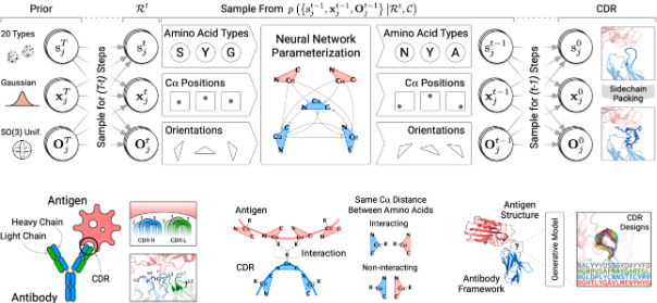
抗体-抗原复合物结构文件,PDB格式
设计模式选择,对于抗原-抗体复合物有4种设计模式可选:
只有在指定Optimize设计模式后,才需要选择改参数,默认值为H_CDR3,一共有6个选项:H_CDR1、H_CDR2、H_CDR3、L_CDR1、L_CDR2、L_CDR3。
1.输出一个结构优化后或构建后的压缩包result.tar.gz。
2.展示不同设计模式的第一个结构优化结果,输出结果分别如下:
(1) Optimize模式,输出输出结果包括:
| 输出文件名称 | 说明 |
|---|---|
| H_CDR1-O1_0000.pdb | O1表示优化次数为1,对应的优化程度很低,序列变化很小 |
| H_CDR1-O2_0000.pdb | O2表示优化次数为2,优化程度低,序列变化小 |
| H_CDR1-O4_0000.pdb | 优化次数为4,优化程度较低,序列变化较小 |
| H_CDR1-O8_0000.pdb | 优化次数为8,优化程度一般,序列变化一般 |
| H_CDR1-O16_0000.pdb | 优化次数为16,优化程度较高,序列变化较大 |
| H_CDR1-O32_0000.pdb | 优化次数为32,优化程度高,序列变化大 |
| H_CDR1-O64_0000.pdb | 优化次数为64,优化程度很高,序列变化很大 |
(2) Fixbb模式,输出输出结果包括:
| 输出文件名称 | 说明 |
|---|---|
| H_CDR1_0000.pdb | 重链CDR1区优化的结构文件 |
| H_CDR2_0000.pdb | 重链CDR2区优化的结构文件 |
| H_CDR3_0000.pdb | 重链CDR3区优化的结构文件 |
| L_CDR1_0000.pdb | 轻链CDR1区优化的结构文件 |
| L_CDR2_0000.pdb | 轻链CDR2区优化的结构文件 |
| L_CDR3_0000.pdb | 轻链CDR3区优化的结构文件 |
(3) Sample_one_CDR模式,输出文件名称与Fixbb 模式相同。
(4) Sample_multi_CDRs模式,输出CDR区进行优化后的结构文件MultipleCDRs_0000.pdb。
Antibody design is conducted based on diffusion probability models and equivalent neural networks, allowing for the generation of antibodies targeting specific antigen structures and optimization of antibody structures and sequences based on antibody-antigen complex structures.
Antibodies are proteins of the immune system that protect the host by binding to specific antigens such as viruses and bacteria. The binding between antibodies and antigens is primarily determined by the complementarity-determining regions (CDRs) of the antibodies. This module is a deep generative model based on diffusion probability models and equivalent neural networks, jointly modeling the sequences and structures of CDRs. This method can explicitly generate antibodies targeting specific antigen structures and is one of the earliest protein structure diffusion probability models. It enables sequence-structure co-design, sequence design with given scaffold structures, and antibody optimization.
Structure file of the antibody-antigen complex in PDB format.
Design mode selection for the antigen-antibody complex with four available options:
This parameter is only required when selecting the Optimize design mode, with a default value of H_CDR3. There are a total of six options: H_CDR1, H_CDR2, H_CDR3, L_CDR1, L_CDR2, L_CDR3.
Outputs a compressed file, result.tar.gz, containing the optimized or constructed structure.
Displays the first structure optimization results for different design modes as follows:
(1)For the Optimize mode, the output includes:
| Output File Name | Description |
|---|---|
| H_CDR1-O1_0000.pdb | O1 indicates optimization at 1, with low optimization level and minimal sequence changes |
| H_CDR1-O2_0000.pdb | O2 indicates optimization at 2, with low optimization level and small sequence changes |
| H_CDR1-O4_0000.pdb | Optimization at 4, with relatively low optimization level and moderate sequence changes |
| H_CDR1-O8_0000.pdb | Optimization at 8, with moderate optimization level and average sequence changes |
| H_CDR1-O16_0000.pdb | Optimization at 16, with relatively high optimization level and significant sequence changes |
| H_CDR1-O32_0000.pdb | Optimization at 32, with high optimization level and substantial sequence changes |
| H_CDR1-O64_0000.pdb | Optimization at 64, with very high optimization level and extensive sequence changes |
(2)For the Fixbb mode, the output includes:
| Output File Name | Description |
|---|---|
| H_CDR1_0000.pdb | Structure file optimized for the heavy chain CDR1 region |
| H_CDR2_0000.pdb | Structure file optimized for the heavy chain CDR2 region |
| H_CDR3_0000.pdb | Structure file optimized for the heavy chain CDR3 region |
| L_CDR1_0000.pdb | Structure file optimized for the light chain CDR1 region |
| L_CDR2_0000.pdb | Structure file optimized for the light chain CDR2 region |
| L_CDR3_0000.pdb | Structure file optimized for the light chain CDR3 region |
(3)For the Sample_one_CDR mode, the output file names are the same as the Fixbb mode.
(4)For the Sample_multi_CDRs mode, the output is the structure file “MultipleCDRs_0000.pdb” after optimizing the CDR regions.
提交GROMACS对应文件,从而进行分子动力学模拟,得到平衡模拟后得到的轨迹文件。
提交模拟体系的gro文件。该文件可以从MD Solvation或者Membrane Solvation模块获取。
提交模拟体系的top文件。该文件可以从MD Solvation或者Membrane Solvation模块获取。
提交模拟体系的itp文件。该文件可以从MD Solvation或者Membrane Solvation模块获取。
提交进行最小化的参数化文件,文件格式为mdp。可以根据GMX MDP Generation模块的Minimization方法或者**GMX MDP Generation (Auto)**生成。
提交进行等压等温的参数化文件,文件格式为mdp。可以根据GMX MDP Generation模块的NPT方法或者**GMX MDP Generation (Auto)**生成。
提交进行平衡模拟的参数化文件,文件格式为mdp。可以根据GMX MDP Generation模块的MD方法或者**GMX MDP Generation (Auto)**生成。
输出结果包括:
| 输出文件名称 | 说明 |
|---|---|
| md.cpt | md模拟断点文件 |
| md.gro | md的分子坐标文件 |
| md.log | md记录文件 |
| md.tpr | md模拟所需的所有初始化数据(分子拓扑、初始结构等) |
| mini.gro | mini运行的分子坐标文件 |
| mini.log | mini运行记录文件 |
| mini.tpr | mini模拟运行所需的所有初始化数据(分子拓扑、初始结构等) |
| npt.gro | npt的分子坐标文件 |
| npt.log | npt记录文件 |
| npt.tpr | npt模拟所需的所有初始化数据(分子拓扑、初始结构等) |
| path.txt | 模拟轨迹文件存储路径,可用于后续分析模块的Path File输入。 |
GROMACS: High performance molecular simulations through multi-level parallelism from laptops to supercomputers. M. J. Abraham, T. Murtola, R. Schulz, S. Páll, J. C. Smith, B. Hess, E. Lindahl, SoftwareX, 1, (2015), 19-25.
Submit corresponding files to GROMACS to perform molecular dynamics simulations and obtain trajectory files after equilibrium simulations.
Submit the gro file of the simulated system. This file can be obtained from the MD Solvation or Membrane Solvation modules.
Submit the top file of the simulated system. This file can be obtained from the MD Solvation or Membrane Solvation modules.
Submit the itp file of the simulated system. This file can be obtained from the MD Solvation or Membrane Solvation modules.
Submit the script file for minimization, in mdp format. This file can be generated using the GMX MDP Generation module with the Minimization method or GMX MDP Generation (Auto).
Submit the script file for NPT (isothermal-isobaric) simulation, in mdp format. This file can be generated using the GMX MDP Generation module with the NPT method or GMX MDP Generation (Auto).
Submit the script file for equilibrium simulation, in mdp format. This file can be generated using the GMX MDP Generation module with the MD method or GMX MDP Generation (Auto).
The output results include:
| Output File Name | Description |
|---|---|
| md.cpt | Checkpoint file for the MD simulation |
| md.gro | Molecular coordinate file for the MD simulation |
| md.log | Log file for the MD simulation |
| md.tpr | All initial data required for the MD simulation (molecular topology, initial structure, etc.) |
| mini.gro | Molecular coordinate file for the minimization run |
| mini.log | Log file for the minimization run |
| mini.tpr | All initial data required for the minimization run (molecular topology, initial structure, etc.) |
| npt.gro | Molecular coordinate file for the NPT simulation |
| npt.log | Log file for the NPT simulation |
| npt.tpr | All initial data required for the NPT simulation (molecular topology, initial structure, etc.) |
| path.txt | Path to store the simulation trajectory files, which can be used as input for the Path File in subsequent analysis modules. |
GROMACS: High performance molecular simulations through multi-level parallelism from laptops to supercomputers. M. J. Abraham, T. Murtola, R. Schulz, S. Páll, J. C. Smith, B. Hess, E. Lindahl, SoftwareX, 1, (2015), 19-25.

SDF File Split是个化合物库文件分割模块,可以将一个大的SDF文件分割为多个SDF文件,支持按文件个数或者分子数目分割,使得分割后的每个SD文件分子数目接近。
小分子库结构文件,SDF格式
生成文件的数目
新生成SDF文件的前缀,默认subset,生成的文件名为:subset1.sdf,subset2.sdf,以此类推。
小分子库结构文件,SDF格式
每个新生成的SD文件包含的分子数目
新生成SDF文件的前缀,默认subset,生成的文件名为:subset1.sdf,subset2.sdf,以此类推。
拆分后的SDF文件列表文件。
SDF File Split is a compound library file splitting module that can divide a large SDF file into multiple SDF files. It supports splitting based on the number of files or the number of compounds, ensuring that the number of molecules in each split SDF file is similar.
Structure file of the small molecule library, in SDF format.
Number of files to generate.
Prefix for the newly generated SDF files, default is “subset”. The generated files will be named as: subset1.sdf, subset2.sdf, and so on.
Structure file of the small molecule library, in SDF format.
Number of compounds to include in each newly generated SDF file.
Prefix for the newly generated SDF files, default is “subset”. The generated files will be named as: subset1.sdf, subset2.sdf, and so on.
List of split SDF files.

Enumerate Stereoisomers是枚举小分子立体异构体的工具,支持顺反异构体和对映异构体两种形式的枚举。立体异构(stereoisomerism)是在有相同分子式的化合物分子中,原子或原子团互相连接的次序相同,但在空间的排列方式不同,与构造异构同属有机化学范畴中的同分异构现象。对所有或未分配的手性原子和键周围的分子进行立体异构体的组合枚举。
小分子结构文件,支持SMILES、MOL、SDF格式。
指定输出文件的名称,支持SDF(.sd)和SMILES格式(.smi)。
枚举模式,包括如下:
UnassignedOnly:只枚举未分配手性原子和键的分子的构型异构体。所有原子和键都分配手性时,选择该选项得到该分子本身。
All:枚举所有立体异构体,包括构型异构和构象异构。
每个分子产生异构体的最大数目。
小分子的smiles字符串,一行一个分子
得到小分子构型异构体的组合SDF文件generated_isomers.sdf。
Enumerate Stereoisomers is a tool for enumerating stereoisomers of small molecules, supporting both cis-trans isomers and enantiomers. Stereoisomerism refers to the phenomenon in organic chemistry where compounds with the same molecular formula have atoms or groups connected in the same order but arranged differently in space, belonging to the category of structural isomerism. It enumerates stereoisomeric combinations for all or unassigned chiral atoms and bonds in a molecule.
The small molecule structure file, supporting SMILES, MOL, and SDF formats.
Specify the name of the output file, supporting SDF (.sd) and SMILES (.smi) formats.
Enumeration modes include:
Maximum number of isomers to generate for each molecule.
SMILES string of the small molecule, one molecule per line.
Obtain a combined SDF file (generated_isomers.sdf) of conformational isomers of small molecules.

SDF Viewer是小分子化合物库的可视化模块,可以针对一个SDF文件生成一个结构和属性可视、可交互、可检索的HTML页面,方便浏览化合物的结构和属性信息。
小分子结构文件,SDF格式
输出HTML文件名,默认为library.html
针对SDF文件生成一个结构和属性可视、可交互、可检索的HTML页面library.html。
The SDF Viewer is a visualization module for small molecule compound libraries. It generates an HTML page that visualizes and makes the structures and properties of compounds in an SDF file interactive and searchable, facilitating the browsing of compound structure and property information.
The small molecule structure file in SDF format.
The output HTML file name, defaulting to library.html.
Generates an interactive and searchable HTML page (library.html) that visualizes the structures and properties of compounds in the SDF file.
HADDOCK v3.0 是一个自下而上的对长期以来被证实的HADDOCK的重新构想,用于生物分子复合物的综合建模。旨在对HADDOCK的核心功能进行模块化和扩展。它能够充分利用模糊的相互作用约束(AIRs)来驱动对接过程。使用蛋白质-蛋白质对接基准5对它进行了评估,并与实时版本(v2.4)进行了比较。该评估是使用每个复合物的真实界面(3.9 Å)进行的,并以成功率表示;在按HADDOCK-score排名的特定解决方案子集中,至少有一个对接解决方案低于指定阈值的BM5目标数量。
用于进行对接的抗体PDB文件,当前仅支持普通双链抗体(需要含有重、轻链)
用于进行对接的抗原PDB文件
注意:
1.每次对接任务仅支持输入一个抗原结构。
2.HADDOCK运行时长约为2-10小时,取决于抗原抗体的体系大小。
输出结果包括:
| 输出文件名称 | 说明 |
|---|---|
| score.csv | 复合物构象的对接能量打分文件 |
| result.tar.gz | 所有复合物构象PDB文件压缩包 |
| cluster_01_model.pdb-cluster_10_model.pdb | 打分前十的复合物构象 |
其中score.csv,包含信息如下:
| 字段名称 | 说明 |
|---|---|
| RANK | 打分排序 |
| Score | 对接能量打分,其中打分值越低,结合能力越强。 |
HADDOCK v3.0 is a bottom-up reimagining of the well-established HADDOCK for comprehensive modeling of biomolecular complexes. It aims to modularize and extend the core functionalities of HADDOCK, leveraging ambiguous interaction restraints (AIRs) to drive the docking process. It has been evaluated against five protein-protein docking benchmarks and compared to the real-time version (v2.4). The evaluation was conducted using the true interfaces (3.9 Å) of each complex and represented in terms of success rates; in a specific subset of solutions ranked by HADDOCK-score, a minimum number of BM5 targets have at least one docking solution below a specified threshold.
PDB file of the antibody used for docking. Currently, only normal antibodies (which must contain both heavy and light chains) are supported.
PDB file of the antigen used for docking.
Note:
The output results include:
| Output File Name | Description |
|---|---|
| score.csv | Docking energy scoring file for complex conformations. |
| result.tar.gz | Compressed archive of all complex conformation PDB files. |
| cluster_01_model.pdb-cluster_10_model.pdb | Top ten complex conformation models before scoring. |
In score.csv, the information is as follows:
| Field Name | Description |
|---|---|
| RANK | Ranking based on scoring. |
| Score | Docking energy score, where lower scores indicate stronger binding capability. |

基于AfCycDesign算法,利用ColabDesign与AlphaFold2等技术,基于模板分子结构骨架的环肽设计,或进行全新环肽设计。测试表明,这种方法能够准确地预测来自单一序列的原生环状肽的结构,在49个案例中,有36个被预测为高置信度的环状肽,pLDDT>0.85,与原生结构相匹配,均方根偏差(RMSD)小于1.5 Å。

本模块存在两种模式FixBB与Hallucination,其中前者表示进行基于模板蛋白(环肽)结构骨架的环肽设计;后者表示进行全新的环肽设计,不参考模板骨架,可设置环肽长度。
。
上传模板蛋白(环肽)结构。注意,环肽长度不能超过100个氨基酸。
指定模板蛋白中用于参考设计的蛋白链标识,如:“B”,如果结构中只有一条链,可以不用指定。
指定设计时固定模板蛋白中的某些位置的氨基酸不变化,如:‘1,5-10’ 将固定模板蛋白中的第1和5至10的氨基酸不变。
指定全新设计的环肽长度,如:20.
指定设计时需要去除的氨基酸类型,如:“C,W”表示设计的环肽不会出现cysteine和Tryptophan。
设计的环肽的三维结构文件result.pdb。
The Cyclic Peptide Design module utilizes the AfCycDesign algorithm in conjunction with technologies such as ColabDesign and AlphaFold2 to design cyclic peptides based on the structural backbone of template molecules or to create entirely new cyclic peptide designs. Tests have shown that this method can accurately predict the structures of native cyclic peptides from a single sequence. Out of 49 cases, 36 were predicted as high-confidence cyclic peptides with pLDDT > 0.85, matching the native structures with a root mean square deviation (RMSD) of less than 1.5 Å.
This module has two modes: FixBB and Hallucination. The former involves designing cyclic peptides based on the template protein (cyclic peptide) structure, while the latter involves designing entirely new cyclic peptides without reference to a template backbone and allows for setting the length of the cyclic peptide.
Upload the template protein (cyclic peptide) structure. Note that the length of the cyclic peptide cannot exceed 100 amino acids.
Specify the protein chain identifier used for reference design in the template protein, e.g., “B”. If there is only one chain in the structure, this can be left unspecified.
Specify the amino acids in the template protein that should remain fixed during design, e.g., ‘1,5-10’ will fix amino acids at positions 1 and 5 to 10 in the template protein.
Specify the length of the newly designed cyclic peptide, e.g., 20.
Specify the types of amino acids to be removed during design, e.g., “C,W” indicates that the designed cyclic peptide will not contain cysteine and tryptophan.
The three-dimensional structure file of the designed cyclic peptide is stored in result.pdb.
基于深度学习技术预测氨基酸突变对蛋白质-蛋白质相互作用的影响。该模块是基于开源的GeoPPI方法开发的,使用蛋白质复合物的深度几何表征来模拟突变对结合亲和力的影响。为了实现几何结构的强大表达能力和预测的稳健性,模块依次采用了两个组件,即一个几何编码器(擅长提取图形特征)和一个梯度增强树(GBT,擅长避免过度拟合)。几何编码器是一个图形神经网络,在相邻的原子上执行神经信息传递,以更新中心原子的表征。它通过一个新的自我监督学习方案进行训练,以产生蛋白质结构的深度几何表示。基于这些对复合物及其突变体的学习表征,GBT从突变数据中学习,以预测相应的结合亲和力变化。
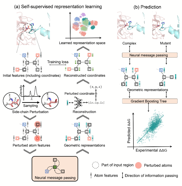
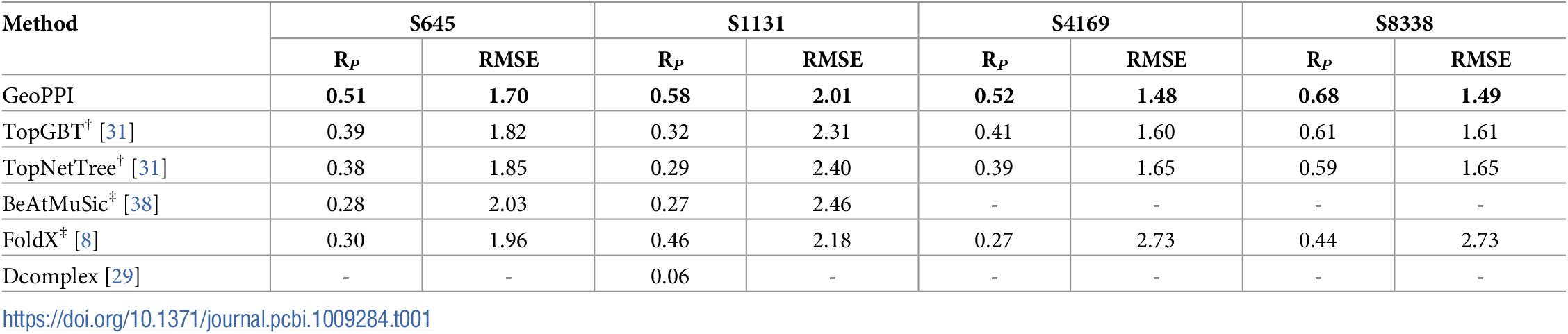
野生型的复合物结构,PDB格式。
突变列表文件,TXT格式,每行包含突变信息,格式如下:
TI17R,EI19R;E_I
AI15R;E_I
每行突变信息及一个相互作用链信息,用分号“;”分隔,其中:
TI17R中的T表示野生型的氨基酸,I表示该氨基酸所在的链,17表示结构文件中该氨基酸的UID编号,R表示突变后的氨基酸。当存在多点突变时,突变信息用逗号(“,”)隔开,如TI17R,EI19R。E_I表示复合物中产生相互作用的蛋白链是E链与I链;相应的,如果是多条链与多条链产生相互作用,如:HL_WV,表示H、L链与W、V链产生相互作用。
需要注意的时突变信息可以时多点或者单点,但是每一行的相互作用链信息只能是一个。
输出结果文件为score.csv,包含信息如下:
| 字段名称 | 说明 |
|---|---|
| Mutation | 突变位点 |
| Chain | 突变点所在的链 |
| Interaction_Chains | 相互作用之间的链名称 |
| deltaEnergy | 该突变引起的结合能量的变化(wildtype-mutant),值越小说明突变后结合越弱,该突变位点对受配体之间结合越重要,单位为kcal/mol。 |
Copyright © 2021 LiuXianggen
Permission is hereby granted, free of charge, to any person obtaining a copy of this software and associated documentation files (the “Software”), to deal in the Software without restriction, including without limitation the rights to use, copy, modify, merge, publish, distribute, sublicense, and/or sell copies of the Software, and to permit persons to whom the Software is furnished to do so, subject to the following conditions:
The above copyright notice and this permission notice shall be included in all copies or substantial portions of the Software.
THE SOFTWARE IS PROVIDED “AS IS”, WITHOUT WARRANTY OF ANY KIND, EXPRESS OR IMPLIED, INCLUDING BUT NOT LIMITED TO THE WARRANTIES OF MERCHANTABILITY, FITNESS FOR A PARTICULAR PURPOSE AND NONINFRINGEMENT. IN NO EVENT SHALL THE AUTHORS OR COPYRIGHT HOLDERS BE LIABLE FOR ANY CLAIM, DAMAGES OR OTHER LIABILITY, WHETHER IN AN ACTION OF CONTRACT, TORT OR OTHERWISE, ARISING FROM, OUT OF OR IN CONNECTION WITH THE SOFTWARE OR THE USE OR OTHER DEALINGS IN THE SOFTWARE.
The Mutation Energy of Binding (GeoPPI) module predicts the effect of amino acid mutations on protein-protein interactions using deep learning techniques. Developed based on the open-source GeoPPI method, this module utilizes deep geometric representations of protein complexes to simulate the impact of mutations on binding affinity. To achieve robust prediction capabilities and powerful geometric structure representations, the module sequentially employs two components: a geometric encoder (proficient at extracting graphical features) and a Gradient Boosting Tree (GBT, adept at preventing overfitting). The geometric encoder is a graph neural network that performs neural message passing on neighboring atoms to update the representation of central atoms. It is trained using a novel self-supervised learning scheme to generate deep geometric representations of protein structures. Based on these learned representations of complexes and their mutants, the GBT learns from mutation data to predict corresponding changes in binding affinity.
The structure of the wild-type complex in PDB format.
A file listing mutations in TXT format, with each line containing mutation information in the following format:
TI17R,EI19R;E_I
AI15R;E_I
Each line contains mutation information and interaction chain information separated by a semicolon “;”. In the mutation information:
It is important to note that mutation information can be single-point or multi-point mutations, but the interaction chain information per line should be only one.
The output result file is score.csv, which includes the following information:
| Field Name | Description |
|---|---|
| Mutation | The mutation site |
| Chain | The chain where the mutation occurs |
| Interaction_Chains | Names of the interacting chains |
| deltaEnergy | The change in binding energy caused by the mutation (wildtype-mutant). A smaller value indicates weaker binding after the mutation, highlighting the importance of the mutation site for the binding between the ligand and receptor, in kcal/mol. |
Copyright © 2021 LiuXianggen
Permission is hereby granted, free of charge, to any person obtaining a copy of this software and associated documentation files (the “Software”), to deal in the Software without restriction, including without limitation the rights to use, copy, modify, merge, publish, distribute, sublicense, and/or sell copies of the Software, and to permit persons to whom the Software is furnished to do so, subject to the following conditions:
The above copyright notice and this permission notice shall be included in all copies or substantial portions of the Software.
THE SOFTWARE IS PROVIDED “AS IS”, WITHOUT WARRANTY OF ANY KIND, EXPRESS OR IMPLIED, INCLUDING BUT NOT LIMITED TO THE WARRANTIES OF MERCHANTABILITY, FITNESS FOR A PARTICULAR PURPOSE AND NONINFRINGEMENT. IN NO EVENT SHALL THE AUTHORS OR COPYRIGHT HOLDERS BE LIABLE FOR ANY CLAIM, DAMAGES OR OTHER LIABILITY, WHETHER IN AN ACTION OF CONTRACT, TORT OR OTHERWISE, ARISING FROM, OUT OF OR IN CONNECTION WITH THE SOFTWARE OR THE USE OR OTHER DEALINGS IN THE SOFTWARE.
ProGen是一种语言模型,可以在大型蛋白质家族中生成具有可预测功能的蛋白质序列,类似于在不同主题上生成语法和语义正确的自然语言句子。该模型基于来自> 19,000个家族的2.8亿个蛋白质序列进行训练,并增加了指定蛋白质属性的控制标签。基于Progen2模型实现,ProGen2模型可扩展到64亿个参数,并在不同的序列数据集上进行训练,这些数据集来自基因组、元基因组和免疫剧目数据库的10亿多个蛋白质。ProGen2模型在捕捉观察到的进化序列的分布、产生新的可行的序列,并预测蛋白质的适应性等方面显示出最先进的性能。
Protein Sequence Generation (ProGen)目前主要功能是基于Reference序列,进行序列的增长(从Reference序列末端开始增长),后续开放其他场景的序列生成功能。
模型类型有2种可选(progen2-large,progen2-xlarge)。
模型信息:
progen2-large,参数数量2.7 Billion,神经网络层数32。
progen2-xlarge,模型参数数量6.4 Billion,神经网络层数32。
作为参考的序列(填序列信息)
注意:不支持多条序列,多条序列会被合并为一条序列。
生成序列的数目。
注意:序列长度不超过1024个氨基酸。
生成的蛋白序列文件result.fasta。
ProGen is a language model designed to generate protein sequences with predictable functions within large protein families, similar to generating syntactically and semantically correct natural language sentences on different topics. The model is trained on 280 million protein sequences from over 19,000 families and incorporates control labels specifying protein attributes. Built upon the Progen2 model, ProGen2 can scale up to 6.4 billion parameters and is trained on over a billion proteins from various sequence datasets sourced from genomes, metagenomes, and immune repertoire databases. ProGen2 demonstrates state-of-the-art performance in capturing the distribution of observed evolutionary sequences, generating novel feasible sequences, and predicting protein adaptability.
Currently, the main function of Protein Sequence Generation (ProGen) is to extend sequences based on a reference sequence (growing from the end of the reference sequence). Additional sequence generation functionalities for other scenarios will be made available in the future.
There are two model options available: progen2-large and progen2-xlarge.
Model details:
The reference sequence for sequence extension (provide sequence information).
Note: Multiple sequences are not supported; multiple sequences will be merged into one sequence.
The number of sequences to generate.
Note: The sequence length should not exceed 1024 amino acids.
The generated protein sequence file is named result.fasta.
Peptide Structure Generation模块只需要输入多肽序列字符或者文件,就能生成多肽的三维或者二维结构的SDF文件。
输入氨基酸序列,每行表示一条多肽,支持同时生成多条多肽。
输出文件名称。
输出多肽结构类型:3d或者2d。
输入氨基酸序列txt文件,与“Peptide Sequence”相同。
其他参数与Peptide Sequence模式相同。
得到多肽三维结构的SDF文件output.sdf。
The Peptide Structure Generation module can generate three-dimensional or two-dimensional structures of peptides in SDF format based on input peptide sequences.
Input amino acid sequences, with each line representing a peptide. Multiple peptides can be generated simultaneously.
Output file name.
Specify the type of peptide structure to generate: 3D or 2D.
Input a text file containing amino acid sequences, similar to the “Peptide Sequence” mode.
Other parameters are the same as in the Peptide Sequence mode.
The output is an SDF file named output.sdf containing the three-dimensional structure of the peptide.
Protein FEP是基于唯信计算自主研发的基于蛋白的自由能微扰算法AlphaFEP,实现了更高效、更精确的蛋白稳定性与蛋白复合物亲和力的相对结合自由能计算,能用于判断单点突变对蛋白稳定性、蛋白复合物结合亲和力的影响。
众多文献报道,FEP方法相比于半经验方法、机器学习方法及GB/PBSA等自由能计算方法,精度更高(例如 http://dx.doi.org/10.1016/j.jmb.2023.168187,见下图,其中PCC代表预测值与SPR实验值的相关性,越高越好)。
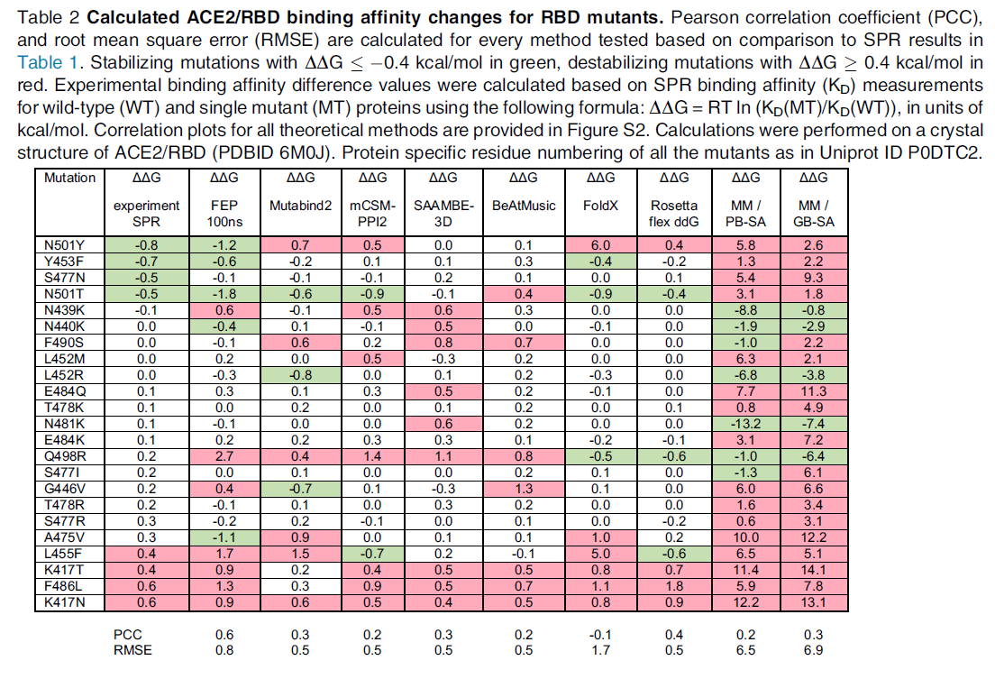
唯信开发的AlphaFEP算法媲美已知的FEP方法,例如Schrodinger的FEP+,并大幅超越其他经典的非FEP方法。下图:结合自由能的预测值与实测值的相关性。
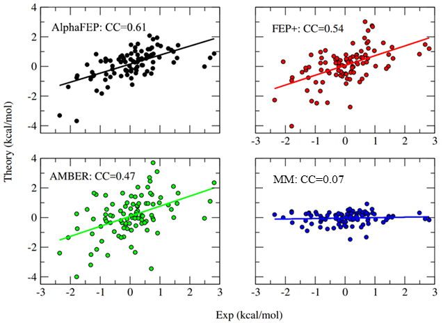
蛋白的结构文件,PDB格式
指定单点突变的位置(如:S52K,S代表野生型氨基酸,52表示该氨基酸在蛋白PDB文件中的索引值,K代表突变后的氨基酸)
指定单点突变类型:稳定性(S)或者结合亲和力(B)
指定单点突变所在的链名称
蛋白的结构文件,PDB格式
多点突变列表文件(.txt),例如:
L28E,H
K30T,H
其中,“L”和“K”是WT;“28”和“30”是PDB文件中的残基ID;“E”和“T”是突变;“H”代表残基的链名。
注意:
输出结果文件为result.txt,包含信息如下:
| 字段名称 | 说明 |
|---|---|
| ligand dG | 配体自由能 |
| complex dG | 复合物自由能 |
| final ddG | 最终突变引起的自由能(结合自由能或折叠自由能)变化,单位为kcal/mol,负值表示蛋白更稳定或结合更强,反之亦然。 |
Jia X, Ge H, Mei Y. Free energy change estimation: The Divide and Conquer MBAR method. J Comput Chem. 2021; 42: 1204–1211. https://doi.org/10.1002/jcc.26533
Protein FEP is a protein-based free energy perturbation algorithm developed by Weixing Computing, which implements the AlphaFEP algorithm for more efficient and accurate calculation of relative binding free energies for protein stability and protein complex affinity. It can be used to assess the impact of single-point mutations on protein stability and protein complex binding affinity.
Numerous studies have shown that FEP methods offer higher accuracy compared to semi-empirical methods, machine learning methods, and GB/PBSA among other free energy calculation methods (e.g., link, as shown in the figure below, where PCC represents the correlation between predicted and experimental values, with higher values indicating better performance).
The AlphaFEP algorithm developed by Weixing Computing rivals established FEP methods like Schrodinger’s FEP+ and significantly surpasses other classical non-FEP methods. The figure below illustrates the correlation between predicted and measured binding free energies.
Structure file of the protein in PDB format.
Specify the position of the single-point mutation (e.g., S52K, where S represents the wild-type amino acid, 52 is the index of the amino acid in the protein PDB file, and K represents the mutated amino acid).
Specify the type of single-point mutation: stability (S) or binding affinity (B).
Specify the chain where the single-point mutation occurs.
Structure file of the protein in PDB format.
File containing a list of multipoint mutations (.txt), for example:
L28E,H
K30T,H
Here, “L” and “K” represent wild-type residues, “28” and “30” are residue IDs in the PDB file, “E” and “T” represent mutations, and “H” denotes the chain name of the residue.
Notes:
The output result file is named result.txt and includes the following information:
| Field Name | Description |
|---|---|
| ligand dG | Ligand free energy |
| complex dG | Complex free energy |
| final ddG | Final change in free energy (binding or folding) caused by the mutation, in kcal/mol. A negative value indicates that the protein is more stable or has stronger binding affinity, and vice versa. |
Jia X, Ge H, Mei Y. Free energy change estimation: The Divide and Conquer MBAR method. J Comput Chem. 2021; 42: 1204–1211. https://doi.org/10.1002/jcc.26533
进行抗体序列突变优化,同时给出序列每个位置20种残基的出现概率值(基于原序列预测)。模块基于Ablang2模型实现,该模型是抗体专用语言模型,为AbLang的升级版,旨在解决抗体序列中的种系偏差(germline bias)问题,从而更有效地支持抗体设计与优化。
抗体多样性主要来源于V(D)J重组、CDR区域的突变以及少量非CDR区域的突变。然而,天然抗体序列中仍有很大部分与种系基因(germline)保持一致,这导致传统语言模型在预训练过程中倾向于“记住”种系序列,而忽视了那些远离种系、但对结合能力至关重要的突变。AbLang2模型的核心目标就是缓解这种种系偏差,提升模型对非种系残基的预测能力,从而更有效地指导抗体工程中的关键突变设计。
AbLang2基于Transformer架构,延续了前代模型AbLang的双组件设计。使用OAS数据库中的非配对(仅重链或轻链)和配对(重链+轻链)抗体序列数据进行训练和微调,提升模型对完整抗体结构的建模能力。
模型预测抗体序列困惑度(perplexity,数值越小表示序列质量越高)的对比,Ablang2效果最佳:
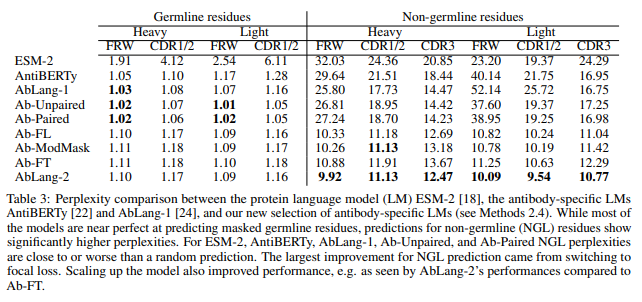
指定需要优化残基的抗体Fv区序列文件,FASTA格式。如果同时有重链Fv(VH)、轻链Fv(VL)序列,通过英文冒号:将序列进行分隔即可,不分先后。如下所示:
>seq1
EVQLLESGGEVKKPGASVKVSCRASGYTFRNYGLTWVRQAPGQGLEWMGWISAYNGNTNYAQKFQGRVTLTTDTSTSTAYMELRSLRSDDTAVYFCARDVPGHGAAFMDVWGTGTTVTVSS
>seq2
QVQLQQSGGELAKPGASVKVSCKASGYTFSSFWMHWVRQAPGQGLEWIGYINPRSGYTEYNEIFRDKATMTTDTSTSTAYMELSSLRSEDTAVYYCASFLGRGAMDYWGQGTTVTVSS:EIVLTQSPGTLSLSPGERATLSCRASQSVSSSFFAWYQQKPGQAPRLLIYGASSRATGIPDRLSGSGSGTDFTLTITRLEPEDFAVYYCQQYDSSAITFGQGTRLEIK
重、轻链同时存在时,后续突变优化过程中,模型会同时考虑重、轻链,符合实际情况。
指定需要突变优化的残基。使用残基位置编号(从1开始),多个残基用逗号分隔,指定残基范围用横杠符号。如:3,10,24-30表示序列中的第3、第10与第24至30号残基,进行突变优化。
在序列中同时存在重、轻链时,需要在残基序号前加上重(H)、轻链(L)标签,如:H5,H8-10,L3表示序列中,重链的第5、第8-10,轻链的第3号残基进行突变优化。
注意:这里定义的待优化残基,会同时应用到Fasta文件中的每条序列(如有不匹配的残基位置,会被自动过滤掉)。
输出优化序列的文件名,Fasta格式,默认为restored.fasta,每条序列仅会产生一条优化的序列。
输出残基概率文件名,CSV格式,默认为restore_probs.csv,输出原序列对应的Positions位置20种残基出现的概率值,以及对应位置优化后的残基。
优化后的序列文件restored.fasta
残基概率文件restore_probs.csv,包含信息如下:
| 字段名称 | 说明 |
|---|---|
| Name | 原序列名称 |
| Chain | 链类型,H或L |
| WT | 序列中的初始残基 |
| POS | AA的位置系引(从1开始) |
| Restored | 序列优化后,该位置的残基 |
| Consensus | 该位置出现概率最大的残基 |
| L,A,G,V… | 该位置每种残基出现的概率 |
注意:Restored的残基并不一定都是Consensus残基,因为概率计算是基于原序列整体计算的,而序列优化是对所有待优化残基进行掩码后(使用*代替原残基),计算可能的最优残基,出现概率会有差异。
Antibody-sequence mutation and optimization are performed while providing, for every position in the sequence, the predicted probability of each of the 20 amino-acid residues (prediction is conditioned on the original sequence). The module is built on Ablang2, an antibody-specific language model that upgrades AbLang and is expressly designed to counteract germline bias in antibody sequences, thereby furnishing stronger support for antibody design and optimization.
Antibody diversity arises chiefly from V(D)J recombination, hypermutation in the CDRs, and a limited number of mutations outside the CDRs. Nevertheless, large tracts of natural antibody sequences remain identical to the germline genes. This causes conventional language models to “memorize” the germline during pre-training and to overlook mutations that deviate from it yet are critical for binding. The central goal of AbLang2 is to mitigate this germline bias and to enhance prediction accuracy for non-germline residues, thus guiding the design of pivotal mutations in antibody engineering.
AbLang2 retains the dual-component architecture of its predecessor and is built on the Transformer framework. It is trained and fine-tuned on both unpaired (heavy- or light-chain-only) and paired (heavy + light) antibody sequences from the Observed Antibody Space (OAS) database, improving its capacity to model intact antibody structures.
Comparison of predicted sequence perplexity (lower values indicate higher sequence quality) confirms that AbLang2 delivers the best performance.

Antibody Fv region sequence file specifying residues to be optimized, in FASTA format.
If both heavy-chain Fv (VH) and light-chain Fv (VL) sequences are provided, simply separate them with an colon :, order does not matter. Example:
>seq1
EVQLLESGGEVKKPGASVKVSCRASGYTFRNYGLTWVRQAPGQGLEWMGWISAYNGNTNYAQKFQGRVTLTTDTSTSTAYMELRSLRSDDTAVYFCARDVPGHGAAFMDVWGTGTTVTVSS
>seq2
QVQLQQSGGELAKPGASVKVSCKASGYTFSSFWMHWVRQAPGQGLEWIGYINPRSGYTEYNEIFRDKATMTTDTSTSTAYMELSSLRSEDTAVYYCASFLGRGAMDYWGQGTTVTVSS:EIVLTQSPGTLSLSPGERATLSCRASQSVSSSFFAWYQQKPGQAPRLLIYGASSRATGIPDRLSGSGSGTDFTLTITRLEPEDFAVYYCQQYDSSAITFGQGTRLEIK
When both heavy and light chains are present, the model will consider them jointly during subsequent mutation optimization, mirroring real-world antibody behavior.
Specify the residues to be optimized. Use residue indices starting at 1; separate individual positions with commas and ranges with a hyphen.
Example: 3,10,24-30 optimizes positions 3, 10 and 24–30.
If the FASTA contains both chains, prefix each index with H (heavy) or L (light).
Example: H5,H8-10,L3 optimizes heavy-chain residues 5 and 8–10, plus light-chain residue 3.
Note: The same Positions list is applied to every sequence in the FASTA; any non-existent positions are silently ignored.
Name of the optimized-sequence file (FASTA format).
Default: restored.fasta.
Each input sequence produces exactly one optimized sequence.
Name of the residue-probability file (CSV format).
Default: restore_probs.csv.
For every position listed in Positions, the file contains the 20-amino-acid probabilities predicted from the original sequence and the residue finally chosen after optimization.
Optimized sequence file: restored.fasta
Residue-probability file: restore_probs.csv
| Column | Description |
|---|---|
| Name | Original sequence identifier |
| Chain | Chain type, H or L |
| WT | Wild-type residue in the original sequence |
| POS | Amino-acid position index (1-based) |
| Restored | Residue after optimization |
| Consensus | Residue with the highest predicted probability |
| A,C,D,E,F,G,H,I,K,L,M,N,P,Q,R,S,T,V,W,Y | Probability of each amino acid at this position |
Note: The Restored residue is not necessarily the Consensus residue.
Probabilities are computed from the original intact sequence, whereas optimization masks all requested positions simultaneously (replacing them with ‘*’) and then infers the globally optimal combination; hence the posterior probabilities can differ.

Structure Clustering是基于分子指纹的小分子结构聚类模块,其采用的聚类方法有Butina或任何其他可用的分层聚类方法。
小分子的结构文件,支持SDF、SMILES格式。
输出文件名称。
在分层聚类过程中生成的聚类的数目。
Butina聚类算法中使用的相似度截断值。
聚类算法,包括如下:
用于计算相似度或者距离的分子指纹类型,包括如下:
分子指纹方式,包括如下:
相似度计算指标,包括如下:
在原有SDF文件中加入聚类编号,得到新的SDF文件output.sdf。
Structure Clustering is a module for clustering small molecule structures based on molecular fingerprints. It employs clustering methods such as Butina or any other available hierarchical clustering method.
The structure file of the small molecule, supported formats include SDF and SMILES.
Name of the output file.
Number of clusters generated during the hierarchical clustering process.
Similarity cutoff value used in the Butina clustering algorithm.
Clustering algorithms available include:
Types of molecular fingerprints used for similarity or distance calculation include:
Types of molecular fingerprint representations include:
Similarity metrics for calculation include:
The original SDF file will be updated with cluster numbers, resulting in a new SDF file named output.sdf.
Sequence Clustering使用DBSCAN算法对多序列比对(MSA)后的结果进行聚类分析,将多序列分为多个cluster类别,并通过可视化模块UMAP进行序列的embedding,并获取二维可视化信息。
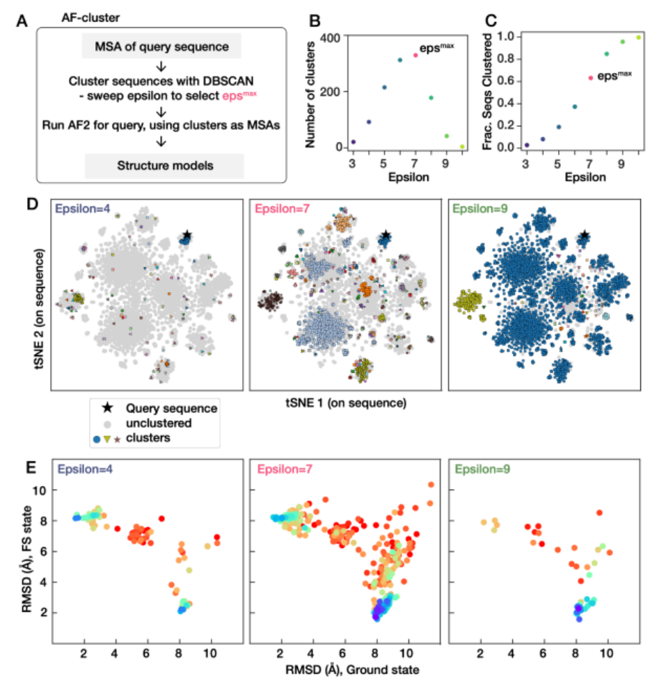
需要聚类序列的多序列比对结果文件(fasta格式),可以由Multiple Sequence Alignmnet模块产生的alignmnet.fasta。
输出结果文件为res_clustering_assignments.tsv,包含信息如下:
| 字段名称 | 说明 |
|---|---|
| SequenceName | 序列名称 |
| sequence | 序列 |
| frac_gaps | 后续序列与参考序列(第一条序列)氨基酸差异(填充‘-’)的比例 |
| dbscan_label | 聚类后的类别标签(如果值为-1表示未分配类别) |
| UMAP 1,UMAP 2 | 二维可视化坐标信息(UMAP 1,UMAP 2对应X,Y坐标) |
Sequence Clustering uses the DBSCAN algorithm to perform cluster analysis on the results of multiple sequence alignment (MSA), dividing multiple sequences into different cluster categories. It utilizes the UMAP visualization module to embed sequences and obtain two-dimensional visualization information.
The file containing the results of multiple sequence alignment (in FASTA format) that need to be clustered. This file can be generated by the Multiple Sequence Alignment module as alignmnet.fasta.
The output result file is res_clustering_assignments.tsv, which includes the following information:
| Field Name | Description |
|---|---|
| SequenceName | Name of the sequence |
| sequence | The sequence itself |
| frac_gaps | Proportion of gaps (‘-’) in the sequence compared to the reference sequence (the first sequence) |
| dbscan_label | Cluster label after clustering (if the value is -1, it means the sequence is unassigned to any cluster) |
| UMAP 1, UMAP 2 | Two-dimensional visualization coordinate information (UMAP 1 corresponds to the X-coordinate and UMAP 2 corresponds to the Y-coordinate) |
Extract Sequence from Structure (PDB2FASTA)模块是从蛋白的PDB文件中将序列提取出来保存为FASTA文件。常规氨基酸序列用单字母表示,其他类型都标注为X。
蛋白的结构文件,PDB格式。
将指定链的序列转存为fasta格式,默认all代表将所有链的序列输出。
控制是否在输出中包含缺失残基。默认为 true 时跳过 SEQRES 记录中存在但结构文件(ATOM/HETATM)中缺失的残基;设置为 false 时将这些 SEQRES 缺失残基包含在输出结果中。
输出序列文件名称,FASTA格式。
得到蛋白的序列文件,默认为seq.fasta。
The Extract Sequence from Structure (PDB2FASTA) module extracts sequences from a protein’s PDB file and saves them as a FASTA file. Conventional amino acid sequences are represented by single letters, while other types are labeled as X.
The protein’s structure file in PDB format.
Specify the chain whose sequence will be saved in FASTA format. Use “all” to output sequences from all chains by default.
Controls whether missing residues are included in the output. Default true skips residues that are recorded in SEQRES but missing from the structure file (ATOM/HETATM records); set false to include these SEQRES missing residues in the output.
Name of the output sequence file in FASTA format.
Obtain the protein sequence file, default name is seq.fasta.
把三字母表示的氨基酸转换为单字母表示。"ASP ILE VAL ASN"转换为 “DIVQ”.
包含三字符氨基酸序列的文本文件
指定输出序列文件的名称,FASTA格式
三字符代表的氨基酸序列,例如:
ASP ILE VAL ASN
指定输出序列文件的名称,FASTA格式
三字母表示的氨基酸转换为单字母,并以序列FASTA格式输出sequence.fasta。
Converts three-letter amino acid representations to single-letter representations. For example, “ASP ILE VAL ASN” is converted to “DIVQ”.
Text file containing sequences of three-character amino acids.
Specify the name of the output sequence file in FASTA format.
Sequence of three-character amino acids, for example:
ASP ILE VAL ASN
Specify the name of the output sequence file in FASTA format.
Converts three-letter amino acid representations to single-letter representations and outputs the sequence in FASTA format as sequence.fasta.

Sequence Translation是DNA序列转换成RNA序列和蛋白序列的工具。
DNA序列文件,FASTA格式
DNA序列,例如:
TTATGACGTTATTCTACTTTGATTGTGCGAGACAATGCTACCTTACCGGTCGGAACTCGATCGGTTGAACTCTATCACGCCTGGTCTTCGAAGTTAGCAC
输出结果包括:
| 输出文件名称 | 说明 |
|---|---|
| prepared_dna.fasta | 转换成DNA的FASTA文件 |
| protein.fasta | 转换成蛋白的FASTA文件 |
| mrna.fasta | 转换成mRNA的FASTA文件 |
Sequence Translation is a tool for converting DNA sequences into RNA sequences and protein sequences.
DNA sequence file in FASTA format.
DNA sequence, for example:
TTATGACGTTATTCTACTTTGATTGTGCGAGACAATGCTACCTTACCGGTCGGAACTCGATCGGTTGAACTCTATCACGCCTGGTCTTCGAAGTTAGCAC
The output includes:
| Output File Name | Description |
|---|---|
| prepared_dna.fasta | FASTA file converted to DNA |
| protein.fasta | FASTA file converted to protein |
| mrna.fasta | FASTA file converted to mRNA |
ESMFold使用大型语言模型从主序列直接推断结构,预测的速度比最先进的方法快60倍,同时能够保持分辨率和准确性。AlphaFold2和其他替代方法使用多序列比对(MSA)和类似蛋白质的模板来实现原子分辨率结构预测的最佳性能获突破性成功;而ESMFold通过利用语言模型的内部表征,只用一个序列作为输入就能生成结构预测。ESMFold与AlphaFold2和RoseTTAFold具有相似的准确性,但ESMFold在探索宏基因组蛋白质的结构空间方面速度更快。
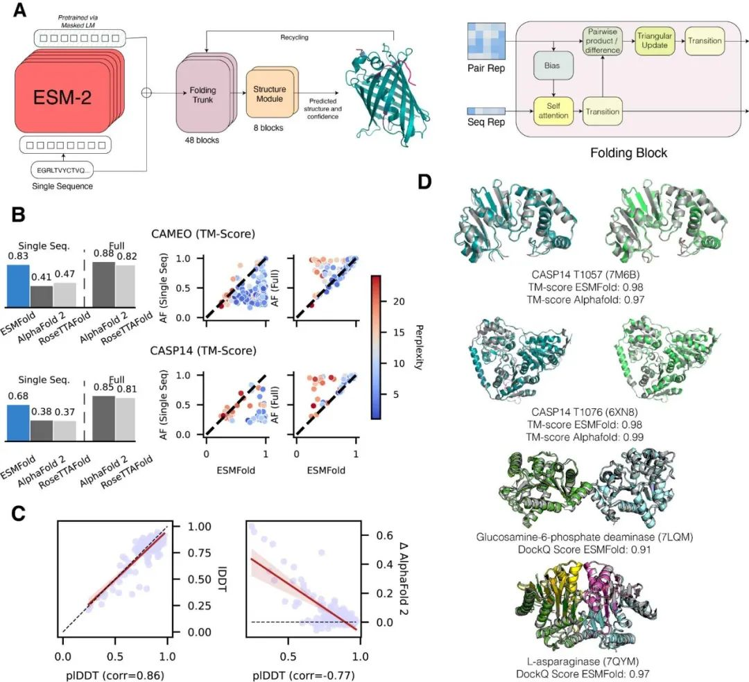
蛋白序列文件,FASTA格式,支持多条序列。
预测复合物,多条链通过英文冒号(:)相连,举例:
>complex
MGITQTPYKVSISGLYLRARV:QVQLQQSGAELARPGASVKMSCKASGYTFTRYTMHWVKQR
每个GPU前向传递中的最大令牌数。这将使较短的序列分组进行批量预测。如果在短序列上发生内存不足问题,降低此值可以有所帮助。
较低的值将导致更低的内存使用,但会降低速度。推荐值:128、64、32。
蛋白序列文件,FASTA格式,多条序列时默认为复合物预测。
输出结果包括:
| 输出文件名称 | 说明 |
|---|---|
| seq1.pdb | 默认输出第一条序列的预测结构。 |
| result.tar.gz | 针对含有多条序列的fasta文件,压缩包中含所有的序列的预测结构。 |
| score.csv | 预测结构的打分,包含结构可靠性指标pLDDT与pTM,pLDDT数值范围在0-100,数值越大表示结构可靠性越高,pTM数值范围在0-1,数值越大表示结构可靠性越高 |
| stdout.txt | 模块的标准输出信息。 |
ESMFold uses a large language model to directly infer structure from primary sequences, with prediction speeds 60 times faster than state-of-the-art methods, while maintaining resolution and accuracy. While AlphaFold2 and other alternative methods achieve breakthrough success in atomic-resolution structure prediction using multiple sequence alignments (MSA) and protein-like templates, ESMFold leverages the internal representation of a language model to generate structure predictions using just one sequence as input. ESMFold exhibits similar accuracy to AlphaFold2 and RoseTTAFold, but is faster in exploring the structural space of macrogenomic proteins.
Protein sequence file in FASTA format, supporting multiple sequences.
For predicting complexes, multiple chains are connected by a colon (:) as shown below:
>complex
MGITQTPYKVSISGLYLRARV:QVQLQQSGAELARPGASVKMSCKASGYTFTRYTMHWVKQR
Maximum number of tokens in each GPU forward pass. This allows grouping of shorter sequences for batch prediction. Lowering this value can help if memory issues occur with short sequences.
A lower value leads to lower memory usage but decreases speed. Recommended values: 128, 64, 32.
Protein sequence file in FASTA format, defaulting to complex prediction for multiple sequences.
The output includes:
| Output File Name | Description |
|---|---|
| seq1.pdb | Default output of the predicted structure for the first sequence. |
| result.tar.gz | For fasta files containing multiple sequences, the compressed file includes predicted structures for all sequences. |
| score.csv | The score of the predicted structure includes the structural reliability indicators pLDDT and pTM. The pLDDT value range is 0-100, and the larger the value, the higher the structural quality. The pTM value range is 0-1, and the larger the value, the higher the structural quality. |
| stdout.txt | Standard output. |
.png)
Retrosynthetic Prediction (AiZynthFinder)是阿斯利康开发的针对小分子的逆反应合成路线预测算法。AiZynthFinder算法基于蒙特卡罗树搜索最终得到可被购买的小分子,用于合成输出分子。树搜索策略采用神经网络方法对已知的反应库进行训练得到。
目标小分子的结构文件,SMILES格式,如:
Cc1cccc(c1N(CC(=O)Nc2ccc(cc2)c3ncon3)C(=O)C4CCS(=O)(=O)CC4)C
输出结果包含逆合成分析结果的层级表示tree.json和逆合成分析的路线图route000.png-route010.png
trees.json把目标分子、反应拆分路径、前体化合物、反应模板等信息都组织在了一棵“树”里面。以下是对trees.json的说明:
"type": "mol",
"smiles": "Cc1cccc(C)c1N(CC(=O)Nc1ccc(-c2ncon2)cc1)C(=O)C1CCS(=O)(=O)CC1",
"is_chemical": true,
"in_stock": false,
"children": [...]
type: "mol" → 说明这是一个分子节点。smiles → 目标化合物的 SMILES 表示。in_stock: false → 表明目标分子不是库存可直接购买的,需要合成。children → 存放对应的反应步骤(reaction)。{
"type": "reaction",
"smiles": "[C:1]...>>...",
"is_reaction": true,
"metadata": {...},
"children": [...]
}
type: "reaction" → 表明这是一个反应。smiles → 带有反应中心标记的反应 SMILES,>> 左边是反应物,右边是产物。metadata → 包含反应模板、来源库(uspto)、匹配次数、概率、反应类别等信息。children → 反应的前体分子(pre-cursors)。{
"type": "mol",
"smiles": "Nc1ccc(-c2ncon2)cc1",
"is_chemical": true,
"in_stock": true
}
in_stock:true→说明这个分子在库存中可以买到,不需要进一步分解。in_stock: false,则它继续有children,表示还能再分解为更基础的前体。reaction→ 拆成前体分子。children)。in_stock: true为止,这条合成路线就闭合了。"scores": {
"state score": 0.994039853898894,
"number of reactions": 2,
"number of pre-cursors": 3,
"number of pre-cursors in stock": 3
},
"metadata": {
"created_at_iteration": 36,
"is_solved": true
}
state score → 预测模型对该路线的置信度。number of reactions → 总共涉及几步反应。number of pre-cursors → 需要多少前体分子。number of pre-cursors in stock → 有多少前体能直接购买。is_solved: true → 说明这条路线是完整可行的合成路径。AiZynthFinder is a tool for retrosynthetic planning. The algorithm is based on a Monte Carlo tree search that recursively breaks down a molecule to purchasable precursors. The tree search is guided by a policy that suggests possible precursors by utilizing a neural network trained on a library of known reaction templates.
Product molecule structure file in SMILES format. Example:
Cc1cccc(c1N(CC(=O)Nc2ccc(cc2)c3ncon3)C(=O)C4CCS(=O)(=O)CC4)C
The output of the retrosynthesis analysis includes a hierarchical representation trees.json and retrosynthesis route diagrams route000.png–route010.png.
The trees.json file organizes the target molecule, reaction decomposition paths, precursor compounds, reaction templates, and related information into a “tree” structure. The explanation is as follows:
{
"type": "mol",
"smiles": "Cc1cccc(C)c1N(CC(=O)Nc1ccc(-c2ncon2)cc1)C(=O)C1CCS(=O)(=O)CC1",
"is_chemical": true,
"in_stock": false,
"children": [...]
}
type: "mol" → Indicates this is a molecule node.smiles → The SMILES representation of the target compound.in_stock: false → The target molecule is not available in stock and must be synthesized.children → Stores the corresponding reaction steps (reaction).{
"type": "reaction",
"smiles": "[C:1]...>>...",
"is_reaction": true,
"metadata": {...},
"children": [...]
}
type: "reaction" → Indicates this is a reaction node.smiles → Reaction SMILES with mapped reaction centers; the left side of >> is reactants, the right side is products.metadata → Contains reaction template, source database (e.g., uspto), occurrence count, probability, classification, and other information.children → The precursor molecules for this reaction.3.Precursor Molecule
{
"type": "mol",
"smiles": "Nc1ccc(-c2ncon2)cc1",
"is_chemical": true,
"in_stock": true
}
in_stock: true → Indicates that this molecule is available in stock and does not need further decomposition.in_stock: false, it will continue to have children, representing further decomposition into more basic precursors.4.Recursive Nesting (Multi-step Reactions)
reaction is decomposed into precursor molecules.children).in_stock: true, completing a feasible synthesis route."scores": {
"state score": 0.994039853898894,
"number of reactions": 2,
"number of pre-cursors": 3,
"number of pre-cursors in stock": 3
},
"metadata": {
"created_at_iteration": 36,
"is_solved": true
}
state score → The confidence score of the predicted route by the model.number of reactions → Total number of reaction steps.number of pre-cursors → Total number of precursor molecules needed.number of pre-cursors in stock → Number of precursors that can be directly purchased.is_solved: true → Indicates that this route is a complete and feasible synthesis path.IgFold是一种基于深度学习的快速预测抗体Fv结构的方法。IgFold由一个预先训练的语言模型和直接预测骨架原子坐标的图网络组成,该语言模型训练了558M个天然抗体序列。IgFold在显著更短的时间内(不到一分钟)预测出与其他方法(包括AlphaFold)相似或更好质量的结构。注:该模块只适合预测可变区构象,如果是全长抗体或者包含多个可变区的抗体等情况,需要使用Protein Structure Prediction (AlphaFold2.3.2)或者Protein Structure Prediction (ESMFold)进行结构预测。
输入抗体Fv区重链和或轻链序列,其中抗体序列名称中必须包含重链标识符:H,Heavy,.H;轻链标识符:L,Light,.L。例如:
>antibody.H
XXXXXX
>antibody.L
XXXXXX
输出文件为预测抗体的结构文件antibody_pred.pdb。
【已知问题】部分预测结构会比输入序列缺失个别氨基酸,请留意!
IgFold, a fast deep learning method for antibody structure prediction. IgFold consists of a pre-trained language model trained on 558M natural antibody sequences followed by graph networks that directly predict backbone atom coordinates. IgFold predicts structures of similar or better quality than alternative methods (including AlphaFold) in significantly less time (under one minute).
Antibody Fv sequence file in FASTA format. The heavy chain sequence name should contain :H, Heavy, or .H. The light chain sequence name should contain :L, Light, or .L. Demo:
>antibody.H
XXXXXX
>antibody.L
XXXXXX
The output file is antibody_pred.pdb, which is a structure file for predicting antibodies.
Part of the predicted structure will be missing individual amino acids compared to the input sequence, please note!
基于神经网络的MHC-I型相互作用预测模型。模型训练是利用亲和力和质谱洗脱配体的数据,预测特定MHC分子结合肽段的亲和力值和肽段的长度,可用于肿瘤新抗原的预测。
蛋白的序列文件,FASTA格式。
输出结果文件为result.csv,包含信息如下:
| 字段名称 | 说明 |
|---|---|
| Seq_ID | 蛋白序列名称 |
| Pos | 肽段在蛋白质序列中的残基编号(从0开始) |
| MHC | MHC分子/等位基因名称 |
| Peptide | 潜在配体的氨基酸序列 |
| Core | 直接与MHC接触的最小的9个氨基酸结合核心 |
| Of | 核心在肽段中的起始位置(如果>0,则该方法预测N-末端突出) |
| Gp | 如有删除,删除的位置 |
| Gl | 如有删除,删除的长度 |
| Ip | 如有插入,插入的位置 |
| Il | 如有插入,插入的长度 |
| Icore | 相互作用核心。这是包括插入和删除的结合核心序列 |
| Identity | 蛋白质标识符,即FASTA条目的名称 |
| Score | 原始预测得分。(EL:质谱洗脱配体,BA:亲和力) |
| %Rank | 预测结合得分与一组随机天然肽相比的排名。此测量不受某些分子固有偏向于更高或更低的预测亲和力的影响。强结合物被定义为具有%rank<0.5的物质,而弱结合物则具有%rank<2。我们建议基于%Rank而不是得分选择候选配体。(EL:质谱洗脱配体,BA:亲和力) |
| Aff(nM) | 亲和力大小 |
| BindLevel | 如果%Rank低于强结合物的指定阈值(默认为0.5%),则将识别肽段为强结合物。如果%Rank高于强结合物的阈值但低于弱结合物的指定阈值(默认为2%),则将识别肽段为弱结合物。(SB:强结合物,WB:弱结合物) |
Nucleic Acids Res. 2020 Jul 2;48(W1):W449-W454.
A neural network-based model for predicting MHC-I interactions. The model is trained using affinity and mass spectrometry-eluted ligand data to forecast the affinity values and lengths of peptides binding to specific MHC molecules. This can be employed for predicting tumor neoantigens.
Protein sequence file in FASTA format.
The output file is result.csv and contains the following information:
| Seq_ID | Protein sequence name |
|---|---|
| Pos | Residue number (starting from 0) of the peptide in the protein sequence. |
| MHC | Specified MHC molecule / Allele name. |
| Peptide | Amino acid sequence of the potential ligand. |
| Core | The minimal 9 amino acid binding core directly in contact with the MHC. |
| Of | The starting position of the Core within the Peptide (if > 0, the method predicts a N-terminal protrusion). |
| Gp | Position of the deletion, if any. |
| Gl | Length of the deletion, if any. |
| Ip | Position of the insertion, if any |
| Il | Length of the insertion, if any |
| Icore | Interaction core. This is the sequence of the binding core including eventual insertions of deletions. |
| Identity | Protein identifier, i.e. the name of the FASTA entry. |
| Score | The raw prediction score. (EL: MS eluted ligand, BA: Binding Affinity) |
| %Rank | Rank of the predicted binding score compared to a set of random natural peptides. This measure is not affected by inherent bias of certain molecules towards higher or lower mean predicted affinities. Strong binders are defined as having %rank<0.5, and weak binders with %rank<2. We advise to select candidate binders based on %Rank rather than Score. (EL: MS eluted ligand, BA: Binding Affinity) |
| Aff(nM) | Affinity value |
| BindLevel | The peptide will be identified as a strong binder if the %Rank is below the specified threshold for the strong binders (by default, 0.5%). The peptide will be identified as a weak binder if the %Rank is above the threshold of the strong binders but below the specified threshold for the weak binders (by default, 2%). (SB: Strong Binder, WB: Weak Binder) |
NPT MDP Generation是生成等温等压(NPT)MDP文件的模块。
Define用于传递预处理器的定义,可以使用任何定义来控制自定义拓扑文件(.top)中的选项。可选择的定义包括以下选项:
模拟中积分方式的选择:md算法。
md是蛙跳法,对符合牛顿公式的运动进行积分。
时间步长,单位为ps。(默认为0.001)
模拟时长,单位为ns。
质心进行操作的组,可以是索引文件中的一个,或者多个组。默认为整个系统。
系统或者系统中各个组质心的操作。(默认为None)
在轨迹文件中写入坐标的频率。(默认为0)
在轨迹文件中写入速度(v)的频率。(默认为0)
在轨迹文件中写入力的频率。(默认为0)
在log文件中写入能量的频率。(默认为50)
在记录能量的文件中写入能量的频率。(默认为100)
输入压缩的轨迹文件的频率。(默认为50)
输入轨迹包含的结构。默认为整个系统。
周期化边界条件设置(默认为xyz)。
原子静电相互作用的计算方法,默认为PME。
库仑力截止距离,单位nm(默认为1.2)
范德华相互作用的计算方法,默认为Cut-off。
LJ或Buckingham截止距离,单位nm(默认为1.2)
能量和压力的长程色散校正方法(默认为EnerPres)。
温度耦合的方法(默认为V-rescale)。
耦合到单独的温度浴的组别,多个组别用空格间隔。
温度耦合时间常数,单位为ps。(默认为0.2)
耦合的参考温度,即动力学模拟的温度,单位为K。(默认为300)
压力耦合的方法(默认为Berendsen)。
压力耦合的各向同性类型。每种类型取一个或多个可压缩性(compressibility)和Coupling Reference Pressure。Time for Pressure Coupling仅允许一个值。(默认为isotropic)
压力耦合的时间常数(所有方向一个值),单位为ps。(默认为2)
耦合的参考压力,单位为bar。(默认为1)
可压缩性(注:这实际上是在bar^-1)对于水在1atm和300k的可压缩性是4.5e-5 bar^-1。所需值的数量由pcoupltype [bar^-1]暗示。
限制类型。(默认为none)
输出文件名称
得到一个计算NPT的MDP文件npt.mdp。
The NPT MDP Generation module is used to generate the MDP file for an isothermal-isobaric (NPT) simulation.
The Define section is used to pass preprocessor definitions that can control options in custom topology files (.top). Available options include:
Choice of integration method in the simulation: md algorithm.
md is the leap-frog algorithm used to integrate motions conforming to Newton’s equations.
Time step size in ps. (Default is 0.001)
Duration of the simulation in ns.
Group(s) for center of mass operations, can be one or multiple groups from the index file. Default is the entire system.
Operations for the system or center of mass of individual groups in the system. (Default is None)
Frequency of writing coordinates to the trajectory file. (Default is 0)
Frequency of writing velocities to the trajectory file. (Default is 0)
Frequency of writing forces to the trajectory file. (Default is 0)
Frequency of writing energy to the log file. (Default is 50)
Frequency of writing energy to the energy file. (Default is 100)
Frequency of inputting compressed trajectory files. (Default is 50)
Structures included in the input trajectory. Default is the entire system.
Setting for periodic boundary conditions (Default is xyz).
Method for calculating atomic electrostatic interactions, default is PME.
Coulomb force cut-off distance in nm. (Default is 1.2)
Method for calculating van der Waals interactions, default is Cut-off.
LJ or Buckingham cut-off distance in nm. (Default is 1.2)
Method for long-range dispersion correction for energy and pressure (Default is EnerPres).
Method for temperature coupling (Default is V-rescale).
Groups to which temperature baths are coupled, multiple groups separated by spaces.
Time constant for temperature coupling in ps. (Default is 0.2)
Reference temperature for coupling in K. (Default is 300)
Method for pressure coupling (Default is Berendsen).
Isotropic type of pressure coupling. Each type takes one or more compressibility and Coupling Reference Pressure values. Time for Pressure Coupling allows only one value. (Default is isotropic)
Time constant for pressure coupling (one value for all directions) in ps. (Default is 2)
Reference pressure for coupling in bar. (Default is 1)
Compressibility (actually in bar^-1). For water at 1 atm and 300K, the compressibility is 4.5e-5 bar^-1. The number of values required is implied by pcoupltype [bar^-1].
Type of constraints. (Default is none)
Output file name.
Generates an MDP file named npt.mdp for the NPT calculation.
Minimize MDP Generation是生成能量优化(Minimization)MDP文件的模块。
模拟中积分方式的选择:cg和steep算法。
cg用于能量最小化的共轭梯度算法,在能量下降最陡峭时,比steep更加高效。
steep用于能量最小化的最陡下降算法。一般在setup的能量最小化中使用。
最小化的最大时间,-1没有最大值。
最大容许力,单位为kJ/(mol·nm)。当最大作用力小于此值,认为最小化过程收敛。(默认为100)
起始步长,单位为nm。(默认为0.01)
在轨迹文件中写入坐标的频率。(默认为50)
在log文件中写入能量的频率。(默认为50)
在记录能量的文件中写入能量的频率。(默认为50)
周期化边界条件设置:
xyz: 在所有方向上使用周期性边界条件
no: 不使用周期性边界条件,忽略box。若要模拟无截止,请将所有Cutoff相关选项和nstlist设置为0。若要在单个MPlrank上实现无截止的最佳性能,请将nstlist设置为0,ns-type=simple.
xy: 仅在x和y方向使用周期性边界条件。这仅适用于 ns-type=grid,并可与墙(walls)结合使用。如果没有墙或只有一面墙,系统在z方向上的大小是无限的,因此不能使用压力糟合或 Ewald求和方法。当使用两个墙时,这些缺点不存在。
原子静电相互作用的计算方法,默认为PME。
指定库仑力阈值,单位为nm。(默认为1.2)
范德华相互作用的计算方法,默认为Cut-off。
LJ或Buckingham截止距离,单位nm。(默认为1.2)
控制拓扑中被转换为刚性完整约束的键类型。典型的刚性水模型没有键,因此不受此关键字的影响。
none:不将键转化为约束.
h-bonds:将与氢原子的键合转换为约束
all-bonds:将所有键转换为约束
h-angles:将所有键转换为约束,并将涉及氢原子的角度转换为键约束
al-angles:将所有结合转换为约束,将所有角度转换为结合约束
输出文件名称
得到一个计算最小化的MDP文件mini.mdp。
The Minimize MDP Generation module is used to generate the MDP file for energy minimization.
Choice of integration method in the simulation: cg and steep algorithms.
cg is the conjugate gradient algorithm used for energy minimization, more efficient than steep when the energy decreases steeply.
steep is the steepest descent algorithm used for energy minimization. Generally used in setting up energy minimization.
Maximum time for minimization, -1 means no maximum.
Maximum allowable force in kJ/(mol·nm). Minimization is considered converged when the maximum force is below this value. (Default is 100)
Initial step size in nm. (Default is 0.01)
Frequency of writing coordinates in the trajectory file. (Default is 50)
Frequency of writing energy to the log file. (Default is 50)
Frequency of writing energy to the energy file. (Default is 50)
Setting for periodic boundary conditions:
Method for calculating atomic electrostatic interactions, default is PME.
Specifies the Coulomb force threshold in nm. (Default is 1.2)
Method for calculating van der Waals interactions, default is Cut-off.
LJ or Buckingham cut-off distance in nm. (Default is 1.2)
Controls which types of bonds in the topology are converted to rigid constraints. Typical rigid water models have no bonds, so they are not affected by this keyword.
Output file name.
Generates an MDP file named mini.mdp for the energy minimization calculation.

MD PDB Prepare是一个在分子动力学模拟前PDB结构处理模块,结合PDBFixer工具对输入PDB文件中的蛋白结果进行修复,再分离出PDB文件中的蛋白结构、小分子结构以及核酸结构。
结构文件,PDB格式。
需要注意体系中若存在配体,其名称不能为*号且必须以HETATM开头。如下所示为正确的小分子结构文件:
HETATM 3767 C1 GOL A 302 -4.671 -11.067 -0.429 1.00 43.56 C
HETATM 3768 O1 GOL A 302 -5.324 -9.793 -0.300 1.00 41.43 O
若体系中有特殊金属原子,只能选AMBER力场。离子需要按照特定书写格式,以下为一些常见原子书写格式:
# Mg2+离子
HETATM 1431 MG MG A 301 -23.030 15.955 -4.315 1.00 47.40 MG
# Mn2+离子
HETATM 1431 MN MN A 301 -23.030 15.955 -4.315 1.00 47.40 MN
# Zn2+离子
HETATM 1431 ZN ZN A 301 -23.030 15.955 -4.315 1.00 47.40 ZN
# Fe2+离子
HETATM 1431 FE2 FE2 A 301 -23.030 15.955 -4.315 1.00 47.40 FE
# Fe3+离子
HETATM 1431 FE3 FE3 A 301 -23.030 15.955 -4.315 1.00 47.40 FE
# Ca2+离子
HETATM 1431 CA CA A 301 -23.030 15.955 -4.315 1.00 47.40 C0
# Cu2+离子
HETATM 1431 CU CU A 301 -23.030 15.955 -4.315 1.00 47.40 CU
其中atom type,residue需要是大写,atom name只需是标准金属离子(可以通过文本编辑器查看书写格式是否相同)。
输出结果包括:
| 输出文件名称 | 说明 |
|---|---|
| protein.pdb | 分离得到体系中蛋白文件 |
| ligand.pdb/ligand_pdb.tar.gz | 分离得到体系中小分子文件或者压缩文件 |
| nucleic_acid.pdb | 分离得到体系中核酸文件 |
| membrane.pdb/lipid_membrane.pdb | 分离得到体系中膜结构 |
MD PDB Prepare is a module for pre-processing PDB structures before molecular dynamics simulations. It uses the PDBFixer tool to repair protein structures in the input PDB file and separates the protein structure, small molecule structure, and nucleic acid structure from the PDB file.
Structure file in PDB format.
It is important to note that if there is a ligand in the system, its name cannot be an asterisk (*) and must start with HETATM. Below is an example of a correct small molecule structure in a file:
HETATM 3767 C1 GOL A 302 -4.671 -11.067 -0.429 1.00 43.56 C
HETATM 3768 O1 GOL A 302 -5.324 -9.793 -0.300 1.00 41.43 O
If the system contains special metal atoms, only the AMBER force field can be selected. Ions need to be written in a specific format. Here are some common atomic writing formats:
# Mg2+ ion
HETATM 1431 MG MG A 301 -23.030 15.955 -4.315 1.00 47.40 MG
# Mn2+ ion
HETATM 1431 MN MN A 301 -23.030 15.955 -4.315 1.00 47.40 MN
# Zn2+ ion
HETATM 1431 ZN ZN A 301 -23.030 15.955 -4.315 1.00 47.40 ZN
# Fe2+ ion
HETATM 1431 FE2 FE2 A 301 -23.030 15.955 -4.315 1.00 47.40 FE
# Fe3+ ion
HETATM 1431 FE3 FE3 A 301 -23.030 15.955 -4.315 1.00 47.40 FE
# Ca2+ ion
HETATM 1431 CA CA A 301 -23.030 15.955 -4.315 1.00 47.40 C0
# Cu2+ ion
HETATM 1431 CU CU A 301 -23.030 15.955 -4.315 1.00 47.40 CU
Where atom type and residue should be in uppercase, and atom name should be the standard metal ion name (you can check the writing format using a text editor).
The output results include:
| Output File Name | Description |
|---|---|
| protein.pdb | Separated protein file from the system |
| ligand.pdb/ligand_pdb.tar.gz | Separated small molecule file or compressed file from the system |
| nucleic_acid.pdb | Separated nucleic acid file from the system |
| membrane.pdb/lipid_membrane.pdb | Separated membrane structure from the system |
可根据起始帧数、结束帧数以及间隔帧数对平衡模拟进行轨迹提取,从而将其转换为GRO或者PDB轨迹文件。
MD模拟后得到的路径文件,可以在GMX MD Run模块或者AlphaAutoMD模块中获取。
文件输出类型:GRO或者PDB。
输出文件是否保留水盒子。
起始位置(单位ps)。
结束位置(单位ps)。
间隔时间,单位ps。
索引文件,ndx格式。对于膜体系的轨迹提取是必填项。
输出结果包括:
| 输出文件名称 | 说明 |
|---|---|
| md_finally.pdb | 最后一帧结构文件 |
| md_center.pdb | PDB格式轨迹文件 |
| md_center.gro | GRO格式轨迹文件 |
The MD Trajectory module allows for the extraction of trajectories from equilibrium simulations based on the starting frame number, ending frame number, and frame interval, converting them into GRO or PDB trajectory files.
Path file obtained after MD simulation, can be obtained from the GMX MD Run module or the AlphaAutoMD module.
File output type: GRO or PDB.
Whether to retain the water box in the output files.
Starting time (in ps).
Ending time (in ps).
Time interval, in ps.
Index file in ndx format. This is a required parameter for extracting trajectories in membrane systems.
The output results include:
| Output File Name | Description |
|---|---|
| md_finally.pdb | Structure file of the final frame |
| md_center.pdb | PDB format trajectory file |
| md_center.gro | GRO format trajectory file |
Protein Protonation是蛋白质子化模块主要是预测每个蛋白残基的pKa并根据指定的pH值判断每个残基的质子化状态。
蛋白的结构文件,PDB格式,该文件可以MD PDB Prepare模块提取得到。
pH值,默认为7。
N端残基质子化状态,只有charge和neutral两个选项,默认charge。
C端残基质子化状态,只有charge和neutral两个选项,默认charge。
自定义残基质子化状态。
预测的含质子化状态的结构文件。
输出结果包括:
| 输出文件名称 | 说明 |
|---|---|
| protein_protonation.pdb | 质子化状态的结构文件 |
| predict_pKa.txt | 含pKa值输出文件 |
The Protein Protonation module is primarily used to predict the pKa of each protein residue and determine the protonation state of each residue based on the specified pH value.
The structure file of the protein in PDB format, which can be obtained from the MD PDB Prepare module.
pH value, default is 7.
Protonation state of the N-terminal residue, with options of charge and neutral, default is charge.
Protonation state of the C-terminal residue, with options of charge and neutral, default is charge.
Customize the protonation state of residues.
Structure file with predicted protonation states.
The output results include:
| Output File Name | Description |
|---|---|
| protein_protonation.pdb | Structure file with protonation states |
| predict_pKa.txt | Output file containing pKa values |
GMX Receptor Parameterization模块根据Gromacs生成受体(包括蛋白或者核酸)的GRO,ITP以及TOP文件。
蛋白结构文件。提交的蛋白质文件最好经过Protein Protonation模块的处理。
若体系中有特殊金属原子,只能选AMBER力场。离子需要按照特定书写格式,以下为一些常见原子书写格式:
# Mg2+离子
HETATM 1431 MG MG A 301 -23.030 15.955 -4.315 1.00 47.40 MG
# Mn2+离子
HETATM 1431 MN MN A 301 -23.030 15.955 -4.315 1.00 47.40 MN
# Zn2+离子
HETATM 1431 ZN ZN A 301 -23.030 15.955 -4.315 1.00 47.40 ZN
# Fe2+离子
HETATM 1431 FE2 FE2 A 301 -23.030 15.955 -4.315 1.00 47.40 FE
# Fe3+离子
HETATM 1431 FE3 FE3 A 301 -23.030 15.955 -4.315 1.00 47.40 FE
# Ca2+离子
HETATM 1431 CA CA A 301 -23.030 15.955 -4.315 1.00 47.40 C0
# Cu2+离子
HETATM 1431 CU CU A 301 -23.030 15.955 -4.315 1.00 47.40 CU
其中atom type,residue需要是大写,atom name只需是标准金属离子(可以通过文本编辑器查看书写格式是否相同)。
核酸结构文件。
力场,默认amber14sb_parmbsc1。以下是各个力场适用于那些情况:
amber03,amber99sb,amber14sb_parmbsc1适合蛋白和核酸的凝聚相模拟。
amber14sb_parmbsc1,charmm36-jul2020适用于脂(膜)。
注意:根据提交的pdb结构选取力场。
水模型,默认spc。
spc:最好用于GROMOS力场。
spce:对纯水体系比SPC、TIP3P都好。
tip3p:最好用于amber。
tip4p:最好用于opls。
输出结果包括:
| 输出文件名称 | 说明 |
|---|---|
| receptor.gro | 受体的分子坐标文件 |
| receptor_itp.tar.gz | 受体平衡模拟时固定原子位置所施加的力 |
| receptor.top | 受体的拓扑文件 |
GROMACS: High performance molecular simulations through multi-level parallelism from laptops to supercomputers. M. J. Abraham, T. Murtola, R. Schulz, S. Páll, J. C. Smith, B. Hess, E. Lindahl, SoftwareX, 1, (2015), 19-25.
The GMX Receptor Parameterization module generates GRO, ITP, and TOP files for receptors (including proteins or nucleic acids) based on Gromacs.
Protein structure file. The submitted protein file is preferably processed through the Protein Protonation module.
If the system contains special metal atoms, only the AMBER force field can be selected. Ions need to be written in specific formats. Below are some common atomic writing formats:
# Mg2+ ion
HETATM 1431 MG MG A 301 -23.030 15.955 -4.315 1.00 47.40 MG
# Mn2+ ion
HETATM 1431 MN MN A 301 -23.030 15.955 -4.315 1.00 47.40 MN
# Zn2+ ion
HETATM 1431 ZN ZN A 301 -23.030 15.955 -4.315 1.00 47.40 ZN
# Fe2+ ion
HETATM 1431 FE2 FE2 A 301 -23.030 15.955 -4.315 1.00 47.40 FE
# Fe3+ ion
HETATM 1431 FE3 FE3 A 301 -23.030 15.955 -4.315 1.00 47.40 FE
# Ca2+ ion
HETATM 1431 CA CA A 301 -23.030 15.955 -4.315 1.00 47.40 C0
# Cu2+ ion
HETATM 1431 CU CU A 301 -23.030 15.955 -4.315 1.00 47.40 CU
Where atom type and residue should be in uppercase, and atom name should match the standard metal ion format (check in a text editor if the writing format is the same).
Nucleic acid structure file.
The default force field is amber14sb_parmbsc1. The applicability of each force field is listed below:
amber03, amber99sb, amber14sb_parmbsc1: suitable for condensed-phase simulations of proteins and nucleic acids.
amber14sb_parmbsc1, charmm36-jul2020: suitable for lipid (membrane) systems.
Note:The force field should be selected according to the submitted PDB structure.
Water model, default is spc.
spc: Best used for the GROMOS force field.
spce: Better for pure water systems compared to SPC and TIP3P.
tip3p: Best used for amber.
tip4p: Best used for opls.
The output results include:
| Output File Name | Description |
|---|---|
| receptor.gro | Molecular coordinate file of the receptor |
| receptor_itp.tar.gz | Force applied to fix atomic positions during receptor equilibrium simulations |
| receptor.top | Topology file of the receptor |
GROMACS: High performance molecular simulations through multi-level parallelism from laptops to supercomputers. M. J. Abraham, T. Murtola, R. Schulz, S. Páll, J. C. Smith, B. Hess, E. Lindahl, SoftwareX, 1, (2015), 19-25.

基于obabel,Antechamber(Ambertool),ACPYPE以及ORCA对小分子进行处理。将小分子的PDB文件根据所需电荷,电荷类型和自旋多重度进行处理,从而生成Gromacs分子动力学模拟所需的GRO和ITP文件。
支持pdb和tar.gz的文件格式。当单个配体时提交pdb文件,多个配体时提交含有pdb的tar.gz文件。该文件最好经过MD PDB Prepare模块处理。
配体分子不能用*号,最好是重新命名成英文名称。
选取计算的电荷类型,默认为bcc电荷。
如设置则配体在该pH环境下加氢;如不设置,按全氢加氢。注意:设置pH后,如果配体电荷不为0,自旋多重度不为1,则需要在Charge Multiplicity设置。
指明要计算的配体文件的电荷和自旋多重度,默认为电荷为0,自旋多重度为1。格式要求:配体文件名称(不包含后缀) 电荷值 自旋多重度,例如提交文件为ligand.pdb、电荷为0、自旋多重度为1,则该栏输入为“ligand 0 1”。
输出结果包括:
| 输出文件名称 | 说明 |
|---|---|
| ligand.gro | 受体的分子坐标文件 |
| ligand_itp.tar.gz | 受体平衡模拟时固定原子位置所施加的力 |
| ligand.mol2/ligand_mol2.tar.gz | 分子结构的mol2文件,多个配体时为tar.gz文件 |
Processing of small molecules is performed based on obabel, Antechamber (Ambertool), ACPYPE, and ORCA. The PDB file of the small molecule is processed according to the desired charge, charge type, and spin multiplicity to generate the GRO and ITP files required for Gromacs molecular dynamics simulations.
Supports file formats of pdb and tar.gz. Submit a pdb file when a single ligand is present, and submit a tar.gz file containing pdb when multiple ligands are present. It is recommended that the file has been processed through the MD PDB Prepare module.
Ligand molecules should not contain asterisks (*), and it is preferable to rename them with English names.
Select the type of charge calculation, with the default being the bcc charge.
If set, hydrogenation of the ligand will occur at the specified pH environment; if not set, full hydrogenation will be applied. Note: when pH is set, if the ligand charge is not 0 and the spin multiplicity is not 1, it needs to be specified in Charge Multiplicity.
Specifies the charge and spin multiplicity of the ligand file to be calculated, with the default charge being 0 and spin multiplicity being 1. Format requirement: ligand file name (excluding the extension) charge value spin multiplicity. For example, if the submitted file is ligand.pdb with a charge of 0 and a spin multiplicity of 1, the input in this field should be “ligand 0 1”.
The output results include:
| Output File Name | Description |
|---|---|
| ligand.gro | Molecular coordinate file of the ligand |
| ligand_itp.tar.gz | Force applied to fix atomic positions during ligand equilibrium simulations |
| ligand.mol2/ligand_mol2.tar.gz | Mol2 file of the molecular structure, a tar.gz file for multiple ligands |
MD MDP Generation是生成平衡模拟(MD)MDP文件的模块。
Define用于传递预处理器的定义,可以使用任何定义来控制自定义拓扑文件(.top)中的选项。可选择的定义包括以下选项:
模拟中积分方式的选择:md算法。
md是蛙跳法,对符合牛顿公式的运动进行积分。
时间步长,单位为ps。(默认为0.001)
模拟时长,单位为ns。
质心进行操作的组,可以是索引文件中的一个,或者多个组。默认为整个系统。
系统或者系统中各个组质心的操作。(默认为None)
在轨迹文件中写入坐标的频率。(默认为0)
在轨迹文件中写入速度(v)的频率。(默认为0)
在轨迹文件中写入力的频率。(默认为0)
在log文件中写入能量的频率。(默认为5000)
在记录能量的文件中写入能量的频率。(默认为1000)
输入压缩的轨迹文件的频率。(默认为1000)
输入轨迹包含的结构。默认为整个系统。
周期化边界条件设置(默认为xyz)。
原子静电相互作用的计算方法,默认为PME。
库仑力截止距离,单位nm。(默认为1.2)
范德华相互作用的计算方法,默认为Cut-off。
LJ势或Buckingham的阈值,单位为nm。(默认为1.2)
能量和压力的长程色散校正方法(默认为EnerPres)。
温度耦合的方法(默认为V-rescale)。
耦合到单独的温度浴的组别,多个组别用空格间隔。
耦合时间常数,每个组别都需要定义温度,-1表示无温度耦合,单位为ps。(默认为0.2)
耦合的参考温度,即动力学模拟的温度,单位为K。(默认为300)
压力耦合的方法(默认为Berendsen)。
压力耦合的各向同性类型。每种类型取一个或多个可压缩性(compressibility)和Coupling Reference Pressure。Time for Pressure Coupling仅允许一个值。(默认为isotropic)
压力耦合的时间常数(所有方向一个值),单位为ps。(默认为2)
耦合的参考压力,单位为bar。(默认为1)
可压缩性(注:这实际上是在bar^-1)对于水在1atm和300k的可压缩性是4.5e-5 bar^-1。所需值的数量由pcoupltype [bar^-1]暗示。
限制类型。(默认为none)
xyz方向的位置限制的力常数,三个数值之间用逗号分隔开,单位为kJ/(mol·nm^2)。例如:500,500,500。
MD运行中距离、角度、二面角限制是否生效:
no表示忽略拓扑文件中的约束信息;
simple表示简单的(每分子)的距离约束;
ensemble表示一个模拟盒中分子系综的距离约束。
约束力权重类型:
equal表示将约束力平分到约束中的所有原子对上;
conservative表示约束力为约束势的导数, 将导致原子对的权重为r^-7.,当Time Constant for Restraints=0时,约束力为保守力。
Dirse mixed采用的方法:
no表示计算约束力时使用时间平均的违反;
yes表示计算约束力时使用时间平均违反与瞬时违反乘积的平方根。
约束的力常数,乘以拓扑文件中相互作用约束给出的Factor即为最终的约束力大小。
限制约束的时间,设置为0时表示MD过程中一直进行约束,单位为ps。
将约束中所有原子对的运行距离和瞬时距离写入能量文件的间隔步数。间隔越小该文件越大。
输出文件名称
生成跑MD的MDP文件md.mdp。
MD MDP Generation is a module for generating the MDP file for equilibrium simulations (MD).
Used to pass definitions to the preprocessor, which can be used to control options in custom topology files (.top). Available options include:
Choice of integration method in the simulation: md algorithm.
md is the leap-frog algorithm for integrating motion conforming to Newton’s equations.
Time step, in ps. (Default is 0.001)
Simulation duration, in ns.
Groups for which center of mass operations will be performed, can be one or multiple groups from an index file. Default is the entire system.
Operations for the system or center of mass of groups in the system. (Default is None)
Frequency of writing coordinates to the trajectory file. (Default is 0)
Frequency of writing velocities to the trajectory file. (Default is 0)
Frequency of writing forces to the trajectory file. (Default is 0)
Frequency of writing energies to the log file. (Default is 5000)
Frequency of writing energies to the energy file. (Default is 1000)
Frequency of inputting compressed trajectory files. (Default is 1000)
Structures included in the input trajectory. Default is the entire system.
Periodic boundary conditions setting. (Default is xyz)
Method for calculating atomic electrostatic interactions, default is PME.
Coulomb force cut-off distance, in nm. (Default is 1.2)
Method for calculating van der Waals interactions, default is Cut-off.
Threshold for LJ potential or Buckingham, in nm. (Default is 1.2)
Method for long-range dispersion correction for energy and pressure. (Default is EnerPres)
Method for temperature coupling. (Default is V-rescale)
Groups to which temperature baths are coupled, multiple groups separated by spaces.
Time constant for temperature coupling, each group defining a temperature needs to be defined, -1 indicates no temperature coupling, in ps. (Default is 0.2)
Reference temperature for coupling, the temperature of the dynamic simulation, in K. (Default is 300)
Method for pressure coupling. (Default is Berendsen)
Isotropic type for pressure coupling. Each type takes one or more compressibility values and a Coupling Reference Pressure. Time for Pressure Coupling allows only one value. (Default is isotropic)
Time constant for pressure coupling (one value for all directions), in ps. (Default is 2)
Reference pressure for coupling, in bar. (Default is 1)
Compressibility (note: this is actually in bar^-1). For water at 1 atm and 300 K, the compressibility is 4.5e-5 bar^-1. The number of values required is indicated by pcoupltype [bar^-1].
Type of constraints. (Default is none)
Force constant for position restraints in the xyz directions, separated by commas, in units of kJ/(mol·nm^2). For example: 500,500,500.
Whether distance, angle, and dihedral restraints are active during MD runs:
no means ignore constraint information in the topology file;
simple means simple (per-molecule) distance constraints;
ensemble means distance constraints for a molecule ensemble in a simulation box.
Type of constraint force weighting:
equal distributes the constraint force equally among all atom pairs in the constraint;
conservative gives the derivative of the constraint potential, leading to a weight of r^-7 for atom pairs, and if Time Constant for Restraints=0, the constraint force is conservative.
Method used by Dirse mixed:
no uses time-averaged violations in computing the constraint force;
yes uses the square root of the time-averaged violation times the instantaneous violation in computing the constraint force.
Force constant for constraints, multiplied by the Factor given by the interaction constraints in the topology file to determine the final constraint force magnitude.
Time for constraints, set to 0 to maintain constraints throughout the MD process, in ps.
Interval steps for writing the running and instantaneous distances of all atom pairs in the constraint to the energy file. Smaller intervals lead to larger files.
Output file name.
Generates the MDP file md.mdp for running MD.
MD Solvation将原有的受配体结构中加入水分子和离子。
输入的受体拓扑文件,可由GMX Receptor Parameterization模块生成。
输入的受体结构文件,可由GMX Receptor Parameterization模块生成。
输入的受体参数(压缩)文件,可由GMX Receptor Parameterization模块生成。
输入的配体结构(压缩)文件,可由GMX Ligand Parameterization模块生成。
输入的配体参数(压缩)文件,可由GMX Ligand Parameterization模块生成。
输出的体系总的拓扑文件
输出的体系总的结构文件
输出的体系参数的(压缩)文件
距离限制,仅当Disre不为no时生效,格式如下所示:
[AtomIndex1] [AtomIndex2] [Type] [Index] [Type] [Low] [Up1] [Up2] [Factor]
其中,AtomIndex1和AtomIndex2为在system.gro的原子编号;Type为施加约束类型,通常设置为1,Type类型见表1;Index是计算顺序;Low、Up1、Up2为原子间限制距离,Low到Up1区间的原子距离是不受限制的,但是不能超过Up2,单位为nm;Factor为因子,将Factor乘以“Disre Force Constant”即为限制力的大小,单位为kJ/mol/nm2。
例如:
10     16      1       0       1      0.0     0.3     0.4     1.0
10     46      1       1       1      0.0     0.3     0.4     1.0
16     22      1       2       1      0.0     0.3     0.4     2.5
表1:GROMACS中三种约束类型对原子对进行限制
| Type Code | 约束类型 | 作用情况 |
|---|---|---|
| 1 | Complex NMR distance restraints | 当Disre Type为ensemble时,即非键相互作用设置为1 |
| 6 | Simple harmonic restraints | 当Disre Type为simple时,即分子内成键相互作用设定,可设为6或者10. |
| 10 | Piecewise linear/harmonic restraints | 当Disre Type为simple时,即分子内成键相互作用设定,可设为6或者10 |
角度限制是两对原子间角度的限制,仅当Disre不为no时生效,格式如下所示:
[AtomIndex1] [AtomIndex2] [AtomIndex3] [AtomIndex4] [Type] [Theta0] [Force Constant] [Multiplicity]
其中,AtomIndex1-AtomIndex2是第一对原子编号;AtomIndex3-AtomIndex4为第二对原子编号;Type在这里无用,定义为1即可;Theta0为约束的角度,单位为deg;Force Constant为约束力常数,单位为kJ/mol;Multiplicity为多重度。
例如
2642 2643 2635 2652 1 67.0 1500 1
二面角限制,仅当Disre不为no时生效,格式如下所示:
[AtomIndex1] [AtomIndex2] [AtomIndex3] [AtomIndex4] [Type] [Label] [Phi] [dPhi] [KFactor] [Power]
其中,AtomIndex1-AtomIndex4为组成二面角的原子编号;Type为约束类型函数,总是为1;Label无效;Phi为参考角,dPhi为超出参考角的角度值,单位为deg;KFactor为因子,将KFactor乘以“Disre Force Constant”即为限制力的大小,单位为 kJ/mol/rad2;Power无效。
例如:
2642 2643 2635 2652 1 67.0 1500 1
约束势函数如下所示:

其中,Φ’为参考角Phi,ΔΦ为超出参考角的值dPhi,K_dihr为限制力的大小KFactor。
输出结果包括:
| 输出文件名称 | 说明 |
|---|---|
| system.gro | 体系的分子坐标文件 |
| system_itp.tar.gz | 体系平衡模拟时固定原子位置所施加的力 |
| system.top | 体系的拓扑文件 |
MD Solvation adds water molecules and ions to the original ligand-bound structure.
Input receptor topology file, can be generated by the GMX Receptor Parameterization module.
Input receptor structure file, can be generated by the GMX Receptor Parameterization module.
Input receptor parameter (compressed) file, can be generated by the GMX Receptor Parameterization module.
Input ligand structure (compressed) file, can be generated by the GMX Ligand Parameterization module.
Input ligand parameter (compressed) file, can be generated by the GMX Ligand Parameterization module.
Output total system topology file.
Output total system structure file.
Output system parameter (compressed) file.
Distance restraints, effective only when Disre is not “no”, formatted as follows:
[AtomIndex1] [AtomIndex2] [Type] [Index] [Type] [Low] [Up1] [Up2] [Factor]
Where AtomIndex1 and AtomIndex2 are atomic indices in system.gro; Type is the type of constraint applied, typically set to 1, see Table 1 for Type codes; Index is the calculation order; Low, Up1, Up2 are the distance limits between atoms, the distance between atoms in the Low to Up1 range is unrestricted but cannot exceed Up2, in nm; Factor is a multiplier, multiplying Factor by the “Disre Force Constant” gives the size of the restraint force, in kJ/mol/nm2.
For example:
10     16      1       0       1      0.0     0.3     0.4     1.0
10     46      1       1       1      0.0     0.3     0.4     1.0
16     22      1       2       1      0.0     0.3     0.4     2.5
Table 1: Three constraint types in GROMACS for atom pairs
| Type Code | Constraint Type | Application |
|---|---|---|
| 1 | Complex NMR distance restraints | Set to 1 for non-bonded interactions when Disre Type is ensemble |
| 6 | Simple harmonic restraints | Set to 6 or 10 for intramolecular bonded interactions when Disre Type is simple |
| 10 | Piecewise linear/harmonic restraints | Set to 6 or 10 for intramolecular bonded interactions when Disre Type is simple |
Angle restraints limit the angle between two pairs of atoms, effective only when Disre is not “no”, formatted as follows:
[AtomIndex1] [AtomIndex2] [AtomIndex3] [AtomIndex4] [Type] [Theta0] [Force Constant] [Multiplicity]
Where AtomIndex1-AtomIndex2 is the first pair of atom indices; AtomIndex3-AtomIndex4 is the second pair of atom indices; Type is not used here, defined as 1; Theta0 is the constrained angle in degrees; Force Constant is the constraint force constant in kJ/mol; Multiplicity is the multiplicity.
For example:
2642 2643 2635 2652 1 67.0 1500 1
Dihedral restraints, effective only when Disre is not “no”, formatted as follows:
[AtomIndex1] [AtomIndex2] [AtomIndex3] [AtomIndex4] [Type] [Label] [Phi] [dPhi] [KFactor] [Power]
Where AtomIndex1-AtomIndex4 are the atomic indices composing the dihedral; Type is always 1; Label is not used; Phi is the reference angle, dPhi is the angle value beyond the reference angle in degrees; KFactor is a factor, multiplying KFactor by the “Disre Force Constant” gives the size of the restraint force in kJ/mol/rad2; Power is not used.
For example:
2642 2643 2635 2652 1 67.0 1500 1
The constraint potential functions are as follows:
Where Φ’ is the reference angle Phi, ΔΦ is the value beyond the reference angle dPhi, and K_dihr is the size of the restraint force KFactor.
The output results include:
| Output File Name | Description |
|---|---|
| system.gro | Molecular coordinate file of the system |
| system_itp.tar.gz | Force applied to fix atomic positions during system equilibrium simulation |
| system.top | Topology file of the system |
通过计算平衡模拟轨迹的均方根偏差(RMSD,Root Mean Square Deviation)和均方根波动(RMSF,Root Mean Square Fluctuation),从而分析结构的稳定性和结构变化情况。
MD模拟后得到的路径文件,可以在**GMX MD Run (GMX2023)模块或者AlphaAutoMD (GMX2023)**模块中获取。
选择分析类型:RMSD或者RMSF(可多选)。
选择需要计算的组别。
自定义需要计算的残基编号,连续参数可用“-”表示,不连续残基用逗号隔开,例如:1-10,15。
自定义需要计算的原子编号,用逗号隔开,例如:CA,O,H。与Custom Resid是交集关系。
索引文件,可由Membrane Solvation模块得到。
输出结果包括:
| 输出文件名称 | 说明 |
|---|---|
| rmsd_result.csv | 所选组别的RMSD的CSV文件 |
| rmsd_result.png | 所选组别的RMSD的PNG文件 |
| rmsd_result.xvg | 所选组别的RMSD的XVG文件 |
| rmsf_*.csv | 所选组别的RMSF的CSV文件 |
| rmsf_*.png | 所选组别的RMSF的PNG文件 |
| rmsf_*xvg. | 所选组别的RMSF的XVG文件 |
| bfac.pdb | PDB中的B-Factor一列为原子RMSF值通过公式<Δr²> = 3B/(8π²)转换得到。 |
By calculating the Root Mean Square Deviation (RMSD) and Root Mean Square Fluctuation (RMSF) of equilibrium simulation trajectories, the stability and structural changes of the system can be analyzed.
The path file obtained after MD simulation, which can be obtained from the GMX MD Run (GMX2023) module or the AlphaAutoMD (GMX2023) module.
Select the type of analysis: RMSD or RMSF (multiple selections possible).
Select the group to be calculated.
Custom residue numbers to be calculated, continuous parameters can be represented by “-”, non-continuous residues are separated by commas, for example: 1-10,15.
Custom atom numbers to be calculated, separated by commas, for example: CA, O, H. This intersects with Custom Resid.
Index file obtained from the Membrane Solvation module.
The output results include:
| Output File Name | Description |
|---|---|
| rmsd_result.csv | CSV file of RMSD for the selected group |
| rmsd_result.png | PNG file of RMSD for the selected group |
| rmsd_result.xvg | XVG file of RMSD for the selected group |
| rmsf_*.csv | CSV file of RMSF for the selected group |
| rmsf_*.png | PNG file of RMSF for the selected group |
| rmsf_*xvg. | XVG file of RMSF for the selected group |
| bfac.pdb | The RMSF values are converted to B-factor values by the formula<Δr^2>=3B/(8π^2). |

传统分子生成模型无法限制特定骨架,限制了分子生成在结构优化中的应用,Scaffold Constrained Generation是一种骨架限制的生成模型,可以限制骨架,指定优化部位,特异性的生成全新分子库。
小分子骨架结构文件,SDF格式。结构中用星号*表示骨架结构上需要连接新结构片段的位置,如下图所示(可使用WeDraw进行结构编辑):
使用WeDraw生成小分子结构文件,SDF格式。
输入带*的小分子SMILES,代表生成部分,其他部分固定不变,支持输入多个。例如:*c1cnc2ccccc2c1
期望生成的分子数目。
最终输出文件的文件名称,默认为scg_results.sdf。
生成优化后的分子库的sdf文件scg_results.sdf。
Traditional molecular generation models cannot restrict specific scaffolds, limiting the application of molecular generation in structure optimization. Scaffold Constrained Generation is a scaffold-constrained generation model that can restrict scaffolds, specify optimization sites, and generate a new molecular library with specificity.
Small molecule scaffold structure file in SDF format. The structure uses an asterisk ‘*’ to indicate the positions on the scaffold structure where new structure fragments need to be connected, as shown in the following figure (WeDraw can be used for structure editing).
Generate small molecule structure file using WeDraw, in SDF format.
Input a small-molecule SMILES string that contains one or more asterisks (*). Each * indicates a position to be generated, while the rest of the structure remains fixed. Multiple asterisks are supported. Demo: *c1cnc2ccccc2c1
The desired number of molecules to generate.
The file name for the final output file, default is scg_results.sdf.
The optimized molecular library is saved in an SDF file named scg_results.sdf.
De novo Generation (Moses)是基于深度学习的分子生成模块,实现了多种主流的分子生成模型,包括字符级循环神经网络,变分自编码器,以及对抗自编码器。
分子生成模型,目前包含以下几种:
char_rnn:Character-level Recurrent Neural Network(CharRNN)字符级循环神经网络。
vae:Variational Autoencoder(VAE)变分自编码器。
aae:Adversarial Autoencoder(AAE)对抗自编码器。
期望生成的分子数目。
采样随机数。
输出结果包括:
| 输出文件名称 | 说明 |
|---|---|
| result.sdf | 生成sdf格式分子库。 |
| result.csv | 生成smiles格式分子库,写入csv文件中,首行列名smiles。 |
De novo Generation (Moses) is a deep learning-based molecular generation module that implements various mainstream molecular generation models, including character-level recurrent neural networks, variational autoencoders, and adversarial autoencoders.
Molecular generation model, currently includes the following:
The desired number of molecules to generate.
The sampling random number.
The output includes:
| Output File Name | Description |
|---|---|
| result.sdf | Generated molecular library in SDF format. |
| result.csv | Generated molecular library in SMILES format, written to a CSV file with the column name “smiles”. |
ProteinMPNN是一种基于深度学习的蛋白质序列设计方法,在天然蛋白质骨架上,ProteinMPNN的序列恢复率为52.4%,而Rosetta为32.9%。在训练过程中加入噪声可以提高蛋白质结构模型的序列恢复率,并且产生的序列可以更稳健地编码它们的结构。X射线晶体学、低温电镜和功能研究也证明了ProteinMPNN的广泛实用性和高准确性,它成功挽救了以前用Rosetta或AlphaFold设计失败的蛋白质单体、环状同源多聚体、四面体纳米颗粒和目标结合蛋白等。
在ProteinMPNN的基础上,Exscientia提出了一种针对抗体结构进行优化的微调逆折叠模型AbMPNN,该模型在抗体序列恢复和结构稳健性方面优于通用蛋白质模型,尤其在超可变区CDR-H3环上有显著改进。
蛋白的结构文件,PDB格式。
指定需要设计的链,多条链用逗号分割,例如:‘A,B’。
输出设计的序列数目。
氨基酸采样温度,T=0.0表示取argmax,T>>1.0表示随机采样。建议的取值为0.1、0.15、0.2、0.25、0.3。较高的值会导致更多的多样性。当需要设计的序列数目较大时,为了获取较多多样性(不重复)序列,建议增大该参数,如设置为0.25
设计残基模式:固定(Fix,指定下一步Position中的残基在设计时保持不变)或者设计(Design,指定下一步Position中的残基可进行设计而其他未指定残基在设计时保持不变)。默认:Fix。
可选参数,用于指定需要操作的氨基酸位置。根据 Position Type 的设置,对选定的氨基酸进行固定或设计。
输入格式为:链名 + 残基编号范围,例如:
A1-10,A30,B12-25
注意:
Chain 与 Position 两个参数必须至少填写一个。可选参数,指定在生成的结果序列中不许出现的氨基酸种类。
可选参数,通过数值控制生成结果中各类型残基的偏向性,文本文件格式,通过残基类型,数值来指定,支持多种残基,每行放置一类残基,如:
H,1.5
D,1.0
C,-1.0
残基偏向性数值意义:
0,表示没有偏向性(默认)小于0,表示少出现大于0,表示多出现0.5,1.0,1.5可选参数,可指定设计时参考的模式。具体含义如下:
Homomer:基于同源多聚体进行序列设计;
use_soluble_mode:基于可溶蛋白模型进行序列设计;
antibody_design:基于抗体优化模型AbMPNN进行序列设计;
ligandMPNN:升级版ProteinMPNN,专门用于模拟蛋白质与非蛋白质组分(如小分子、核苷酸和金属)之间的相互作用。
cyclic:环肽的逆折叠序列设计
MPNN预测的每个位置的概率:0为不进行预测,1为进行预测。
输出结果文件result.fasta,包含最终设计的序列。
序列名称中包含多个评价指标:
complex.fastaSave Probablility时,输出probs.tar.gz,包含预测的每个位置的概率。指定参数--ligandMPNN时,result.fasta序列名称包含指标:
--pack_side_chains时,输出设计后的结构打包文件packed_side_chains.tar.gz,包含最终设计的序列对应的复合物结构PDB文件。ProteinMPNN is a deep learning-based protein sequence design method that achieves a sequence recovery rate of 52.4% on natural protein scaffolds, compared to 32.9% for Rosetta. Adding noise during the training process can improve the sequence recovery rate of the protein structural model, and the resulting sequences can more robustly encode their structures. X-ray crystallography, cryo-electron microscopy, and functional studies have also demonstrated the wide applicability and high accuracy of ProteinMPNN, which has successfully rescued previously failed protein monomers, cyclic homooligomers, tetrahedral nanoparticles, and target-binding proteins designed using Rosetta or AlphaFold.
On top of ProteinMPNN, Exscientia has introduced a fine-tuning inverse folding model called AbMPNN specifically tailored for optimizing antibody structures. This model outperforms general protein models in antibody sequence recovery and structural robustness, particularly showing significant improvements in the highly variable CDR-H3 loop region.
Protein structure file in PDB format.
Specify the chain to be designed, multiple chains are separated by spaces, for example: ‘A,B’.
Output the number of sequences designed.
Amino acid sampling temperature, T=0.0 means argmax, T>>1.0 means random sampling. The suggested values are 0.1, 0.15, 0.2, 0.25, 0.3. Higher values result in more diversity. When the required number of designed sequences is large, increase this parameter—e.g., set it to 0.25—to obtain greater sequence diversity and reduce duplicates.
Residue Design Mode: Fixed (Fix, specifying that the residues in the next Position step remain unchanged during design) or Design (Design, specifying that the residues in the next Position step can be designed while other unspecified residues remain unchanged during design). Default: Fix.
An optional parameter specifying the amino acid positions to operate on. Depending on the Position Type setting, the selected residues will be either fixed or designed.
Input format: chain name + residue number range, for example:
A1-10,A30,B12-25
Notes:
Chain and Position must be provided.Optional parameter specifying the types of amino acids that are not allowed to appear in the generated sequence.
Optional parameter to control the bias of different residue types in the generated results. The text file format specifies residue_type,value, supporting multiple residues, with one residue per line, for example:
H,1.5
D,1.0
C,-1.0
Meaning of residue bias values:
0 indicates no bias (default)<0 indicates less frequent appearance>0 indicates more frequent appearance0.5, 1.0, 1.5Optional parameter specifying the reference mode for design. Specific meanings are as follows:
Homomer: Sequence design based on homologous oligomers;
use_soluble_mode: Sequence design based on soluble protein models, namely SolMPNN, the MPNN model trained exclusively on soluble protein data.
antibody_design: Sequence design based on the antibody optimization model AbMPNN, the model obtained by fine-tuning the ProteinMPNN model using antibody structure data.
ligandMPNN: Enable small-molecule (ligand) interaction modeling.
cyclic: Inverse folding sequence design for cyclic peptides.
When none of the above options are selected, the default ProteinMPNN model will be used, which is trained on all protein structures from the PDB database.
Probability of each position predicted by MPNN: 0 for no prediction, 1 for prediction.
The output file is result.fasta and contains the final design sequence.
The sequence names contain multiple evaluation metrics:
Score: This is the probability score for designed residues, where a lower score is generally better. The probability score is the negative logarithm (-logP) of the average probability of the designed residues, so a lower score indicates a higher average probability value.
Global Score: This is the overall probability score for all residues in the sequence, where a lower score is generally better. The probability score is the negative logarithm (-logP) of the average probability of the designed residues, so a lower score indicates a higher average probability value.
seq_recovery: the sequence recovery rate (the degree of similarity to the original sequence) is between 0 and 1, the higher the higher the similarity to the original sequence.
Save Probability , the output probs.tar.gz contains the predicted probability for each position.--ligandMPNN, the sequence names in result.fasta contain the following metrics:1.overall_confidence: Confidence score for the full designed sequence, ranging from 0 to 1.0. A higher value indicates higher sequence confidence.
2.ligand_confidence: Confidence score for all designed residues of the sequence, ranging from 0 to 1.0. A higher value indicates higher confidence in the designed part of the sequence.
3.seq_rec: Sequence recovery rate (similarity to the original sequence), ranging from 0 to 1. A higher value indicates greater similarity to the original sequence.
Outputs the best (highest-scoring) complex sequence complex.fasta.
When specifying the parameter --pack_side_chains, outputs the side-chain-packed structure file packed_side_chains.tar.gz, which contains the PDB structure files of the final designed complex corresponding to the designed sequences.

FASTA File是一个指定FASTA文件的模块,可以用于其他模块的输入。会对FASTA文件的有效性进行判断。
上传FASTA文件
输出一个对应的FASTA文件,会对文件的有效性进行判断。
FASTA File is a module for specifying fasta file which could used for other modules input.
input FASTA file
Generate a corresponding FASTA file and validate its effectiveness.
AlphaShape(简称AlphaS)是一种构象表征与识别算法,可以基于分子的三维空间形状和药效团等药学特征比较进行高通量的虚拟筛选,可以最大化区分海量化合物中与已知活性分子相似的活性化合物(筛选的化合物库分子可使用AlphaConf进行构象生成)。也可用于蛋白质结构域匹配以指导蛋白质设计。
通过创造性地在高斯函数表征方式之上融合深度学习技术,AlphaShape虚拟筛选的计算精度已经领先同超越主流商业算法(例如Schrodinger的Phase,OpenEye的ROCS),在DUD-E标准数据集的测试中,虚拟筛选的AUC值达到了0.837(对比Phase与ROCS的0.663及0.696)。
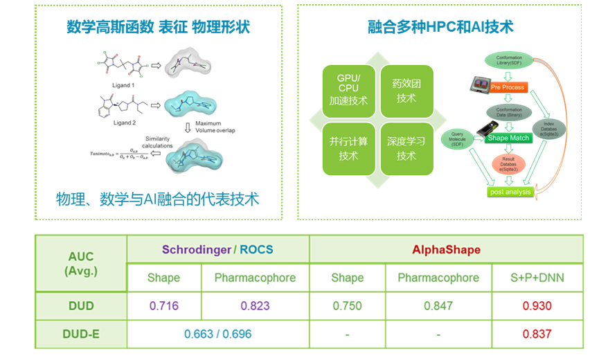
通过采用高性能计算(HPC)技术,特别是NVIDIA的GPU加速技术,目前在搜索或筛选速度上都领先同领域商业软件。以小分子化合物筛选为例,使用一块GPU卡,数小时即可筛完全世界所有的现货商业化合物库的数千万分子,一天可高通量虚拟筛选上亿个化合物分子。
目前已被多家合作药企用于虚拟筛选并成功发现生物活性分子。目前已被合作药企用于虚拟筛选并成功发现生物活性分子。
除了高精度之外,AlphaShape 还充分利用了GPU的能力。 一张GPU卡每天可以筛选大约 5000万种化合物。
输入查询分子文件,SDF格式
小分子的构象库文件,由AlphaConf模块产生,AC.GZ格式
小分子的片段库文件,由AlphaConf模块产生,AUX.GZ格式
输出和每个查询分子相似度排名前n个分子,默认100。
是否对输入的查询分子产生3D构象,True 表示生成,当输入分子是2D结构时可用,False表示不生成,直接使用输入分子的3D结构。
输出最终相似度命中化合物的文件名称,SDF格式,默认文件名为hits.sdf
输入查询分子文件,SDF格式
系统内置的小分子化合物数据库,可多选。
输出和每个查询分子相似度排名前n个分子,默认100。
是否对输入的查询分子产生3D构象,True 表示生成,当输入分子是2D结构时可用,False表示不生成,直接使用输入分子的3D结构。
输出最终相似度命中化合物的文件名称,SDF格式,默认文件名为hits.sdf
输出结果包括:
| 输出文件名称 | 说明 |
|---|---|
| result.csv | 相似度值信息,包含查询分子名称与库中分子名称。 |
| hits.sdf | 筛选相似度最高的n个化合物。多个查询分子时,这个文件是多个查询分子命中化合物合并去重后的结果。 |
| result/AA-173-40757587.sdf | 查询分子对应的命中化合物。每个查询分子都会生成一个对应的包含top n个命中化合物的文件 |
其中result.csv,包含信息如下:
| 字段名称 | 说明 |
|---|---|
| querymol | 查询分子化合物名称 |
| confdb | 化合物库名称 |
| molname | 命中化合物名称 |
| Total Similarity | 3D相似度值 |
AlphaShape (AlphaS for short) is a conformation representation and recognition algorithm that enables high-throughput virtual screening based on the three-dimensional spatial shape and pharmacophoric features of molecules. It maximizes the differentiation of active compounds similar to known active molecules from a large number of compounds (the molecules in the compound library for screening can be generated using AlphaConf). It can also be used for protein domain matching to guide protein design.
By creatively integrating deep learning technology on top of Gaussian function representation, AlphaShape’s virtual screening computational accuracy has surpassed and outperformed mainstream commercial algorithms (such as Schrodinger’s Phase, OpenEye’s ROCS). In testing on the DUD-E standard dataset, the AUC value of virtual screening reached 0.837 (compared to Phase and ROCS at 0.663 and 0.696).
By employing high-performance computing (HPC) technology, especially NVIDIA’s GPU acceleration technology, AlphaShape currently leads in search or screening speed compared to commercial software in the field. For example, in small molecule compound screening, using a single GPU card, it is possible to screen tens of millions of molecules in commercial compound libraries worldwide in a few hours, and conduct high-throughput virtual screening of billions of compound molecules in a day.
It has been used by several collaborative pharmaceutical companies for virtual screening and successful discovery of bioactive molecules. In addition to high accuracy, AlphaShape fully leverages the capabilities of GPUs. A single GPU card can screen approximately 50 million compounds per day.
Input file of query molecules in SDF format.
File of conformation libraries for small molecules, generated by the AlphaConf module, in AC.GZ format.
File of fragment libraries for small molecules, generated by the AlphaConf module, in AUX.GZ format.
Output the top N molecules ranked by similarity to each query molecule, default is 100.
Whether to generate 3D conformations for the input query molecules. True for generation, useful when the input molecules are in 2D structure; False for direct use of the input molecules’ 3D structures.
File name for the final hit compounds based on similarity, in SDF format, default file name is hits.sdf.
Input file of query molecules in SDF format.
System’s built-in small molecule compound database, multiple selections allowed.
Output the top N molecules ranked by similarity to each query molecule, default is 100.
Whether to generate 3D conformations for the input query molecules. True for generation, useful when the input molecules are in 2D structure; False for direct use of the input molecules’ 3D structures.
File name for the final hit compounds based on similarity, in SDF format, default file name is hits.sdf.
The output includes:
| Output File Name | Description |
|---|---|
| result.csv | Information on similarity values, including query molecule names and library molecule names. |
| hits.sdf | Top N screened compounds based on similarity. For multiple query molecules, this file is the merged and deduplicated result of top N hit compounds for each query molecule. |
| result/AA-173-40757587.sdf | Hit compounds corresponding to the query molecule. A file containing the top N hit compounds is generated for each query molecule. |
In result.csv, the information includes:
| Field Name | Description |
|---|---|
| querymol | Query molecule name |
| confdb | Compound library name |
| molname | Hit compound name |
| Total Similarity | 3D similarity value |

File Convert是基于RDKit对分子文件格式之间进行转换的模块。支持的输入文件格式为:SD(.sdf、.sd)、SMILES(.smi、.csv、.tsv、.txt)、PDB(.pdb)、mol2。支持的输出文件格式为:SD(.sdf、.sd)、SMILES(.smi)、PDB(.pdb)。
小分子结构文件,SD、SMILES、PDB或mol2格式。
输出文件名。更改文件扩展名。
输入SDF文件转换成SMILES格式output.smi文件。
The File Convert module is designed to convert molecular file formats using RDKit. Supported input file formats include: SD (.sdf, .sd), SMILES (.smi, .csv, .tsv, .txt),PDB(.pdb), mol2. Supported output file formats include: SD (.sdf, .sd), SMILES (.smi), PDB (.pdb).
Input file containing the molecular structure in SDF or SMILES format.
Name of the output file. Change the file extension as needed.
Convert the input SDF file to SMILES format and save it as output.smi.
Metabolism Site Prediction模块为预测小分子被CYP450代谢的代谢位点。模型对小分子的每个原子进行评估被代谢的可能性,并通过打分排序。支持的小分子输入文件格式为:SD(.sdf、.sd)、SMILES(.smi)。
小分子结构文件,SDF或者SMILES格式。
输出结果包括:
| 输出文件名称 | 说明 |
|---|---|
| molecule_1_atomNumbers.png | 原子编号图片 |
| molecule_1_heteroAtoms.png | P450代谢酶(CYP3A4)预测结果图 |
| molecule_1_heteroAtoms1A2.png | P450代谢酶(CYP1A2)预测结果图 |
| molecule_1_heteroAtoms2C19.png | P450代谢酶(CYP2C19)预测结果图 |
| molecule_1_heteroAtoms2C9.png | P450代谢酶(CYP2C9)预测结果图 |
| molecule_1_heteroAtoms2D6.png | P450代谢酶(CYP2D6)预测结果图 |
| results.csv | 评估被代谢可能性的csv文件 |
| results.html | 评估被代谢可能性的html文件 |
其中results.html,包含如下信息:
| Field Name | Description |
|---|---|
| Rank | 排序 |
| Atom | 原子类型和序号 |
| Score | 最终的打分,也是排序的标准,打分越低,排名越前,被代谢的可能性越高。 |
| Energy | 能量值,基于DFT计算以及原子匹配得到的原子激活的能量值。是打分Score的重要参考项。 |
| Accessibility | 原子到分子中心的相对拓扑距离。 |
The Metabolism Site Prediction module is used to predict the metabolism sites of small molecules by P450 enzymes. The model evaluates the likelihood of each atom in the small molecule being metabolized and ranks them based on scores. Supported input file formats for small molecules include: SD (.sdf, .sd) and SMILES (.smi).
Input file containing the small molecule structure in SDF or SMILES format.
The output includes:
| Output File Name | Description |
|---|---|
| molecule_1_atomNumbers.png | Image showing atom numbering |
| molecule_1_heteroAtoms.png | Prediction results for P450 enzyme (CYP3A4) |
| molecule_1_heteroAtoms1A2.png | Prediction results for P450 enzyme (CYP1A2) |
| molecule_1_heteroAtoms2C19.png | Prediction results for P450 enzyme (CYP2C19) |
| molecule_1_heteroAtoms2C9.png | Prediction results for P450 enzyme (CYP2C9) |
| molecule_1_heteroAtoms2D6.png | Prediction results for P450 enzyme (CYP2D6) |
| results.csv | CSV file evaluating the likelihood of metabolism |
| results.html | HTML file evaluating the likelihood of metabolism |
The results in results.html include the following information:
| Field Name | Description |
|---|---|
| Rank | Ranking |
| Atom | Atom type and number |
| Score | Final score, also the sorting criterion. The lower the score, the higher the ranking, indicating a higher likelihood of metabolism. |
| Energy | Energy value based on DFT calculations and atomic activation energy obtained from atomic matching. An important reference for the score. |
| Accessibility | Relative topological distance of the atom to the molecular center. |

Toxic Fragment Identification模块用于识别小分子的毒效片段,从文献中收集了大量的毒效片段构成毒效片段库,利用子结构匹配方法,实现对化合物库中每个分子进行毒效片段匹配,并通过不同颜色区分。
小分子结构文件,SDF或者SMILES格式。
得到化合物库中与小分子毒效片段匹配的output.xlsx文件,并通过不同颜色区分毒性片段。
output.xlsx包括如下信息:
| 字段名称 | 说明 |
|---|---|
| Smiles | 分子的smiles |
| Image | 分子的化学结构图片,包括毒效片段的匹配。 |
| MolName | 分子名称 |
| Smarts | 毒效片段的Smarts |
| Bad_type | 毒性类型 |
| BadNum | 毒性数量 |
| Literature | 参考文献 |
| Colors | 毒效片段匹配颜色 |
Bad_type毒性类型,包括如下:
Potential_electrophilic_agents,Inpharmatica,Idiosyncratic_toxicity_(RM_formation),Non-genotoxic_carcinogenicity,Endocrine_disruption,MLSMR,AlphaScreen-HIS-FHs,AlphaScreen-FHs,Nonbiodegradable_compounds,Acute_Aquatic_Toxicity,AlphaScreen-GST-FHs,LINT,Promiscuity,LD50_mo_oral,Reactive,_unstable,_toxic,Skin_sensitization,Chelating_agents,Genotoxic_carcinogenicity,_mutagenicity,Developmental_and_mitochondrial_toxicity,PAINS,Hepatotoxicity_Nephrotoxicity,SMARTSfilter,Hepatotoxicity,Toxtree,Myelotoxicity
The Toxic Fragment Identification module is used to identify toxic fragments of small molecules. A large library of toxic fragments has been collected from the literature. Using a substructure matching method, this module matches toxic fragments in each molecule of the compound library and distinguishes them with different colors.
Small molecule structure file in SDF or SMILES format.
Obtain the output.xlsx file that matches toxic fragments in the compound library with the small molecule, color-coding the toxic fragments.
The output.xlsx includes the following information:
| Field Name | Description |
|---|---|
| Smiles | Molecular SMILES |
| Image | Chemical structure image of the molecule, including the matched toxic fragments. |
| MolName | Molecule name |
| Smarts | Toxic fragment SMARTS |
| Bad_type | Type of toxicity |
| BadNum | Number of toxicities |
| Literature | Literature reference |
| Colors | Colors for toxic fragment matches |
The Bad_type toxicity types include:
Potential_electrophilic_agents, Inpharmatica, Idiosyncratic_toxicity_(RM_formation), Non-genotoxic_carcinogenicity, Endocrine_disruption, MLSMR, AlphaScreen-HIS-FHs, AlphaScreen-FHs, Nonbiodegradable_compounds, Acute_Aquatic_Toxicity, AlphaScreen-GST-FHs, LINT, Promiscuity, LD50_mo_oral, Reactive,_unstable,_toxic, Skin_sensitization, Chelating_agents, Genotoxic_carcinogenicity,_mutagenicity, Developmental_and_mitochondrial_toxicity, PAINS, Hepatotoxicity_Nephrotoxicity, SMARTSfilter, Hepatotoxicity, Toxtree, Myelotoxicity
AlphaRNA是Wecomput开发的程序,可以有效地共同优化CAI(Codon Adaption Index)和MFE(Minimum free energy)/AUP(Average unpaired probability)。AlphaRNA提供了一种基于DFA图进行Motif约束的方法,该方法在不明显增加计算量的同时,隐式地将约束加入到密码子优化地过程中以获得更好的密码子偏好性和更稳定的二级结构,以优化其表达量和半衰期、抗体滴度等。可以支持任意数量和长度的序列。

所需要优化的编码区氨基酸序列,例如:
MDIDPYKEFGATVELLSFLPSDFFPSVRDLLDTASALYREALESPEHCSPHHTALRQAIL
要限制(避免出现在优化后序列中)的酶切位点,可多选。
需要限制的Motif序列,可指定多个,可手动输入不在列表中的新序列,使用空白符分隔。
CAI的lambda系数,正值越大能够调大结果中的CAI, 可设置多个,可为负值,负值越大表示越降低CAI。
GC碱基比例(GCR)的lambda系数,正值越大能够调大结果中的GCR, 可设置多个,可为负值,负值越大表示越降低GCR。
输出结果文件为result.csv,包含信息如下:
| 字段名称 | 说明 |
|---|---|
| lambda_cai | CAI的lambda系数 |
| lambda_gcr | GCR的lambda系数 |
| full_sequence | 优化后的序列 |
| CAI | 密码子适应指数 |
| AUP | 平均未配对率 |
| GCR | GC碱基比例 |
| MFE Structure | 最小自由能二级结构 |
| dG(MFE)[kcal/mol] | 最小自由能 |
AlphaRNA is a Wecomput-developed program that efficiently co-optimize both Codon Adaption Index (CAI) and Minimum free energy (MFE)/Average unpaired probability (AUP).It provides a method for motif-constrained codon optimization based on DFA graphs, which implicitly incorporates constraints into the codon optimization process to achieve better codon preferences and more stable secondary structures, optimizing expression levels, half-life, antibody titers, etc., without significantly increasing computational complexity. This method supports sequences of arbitrary numbers and lengths.
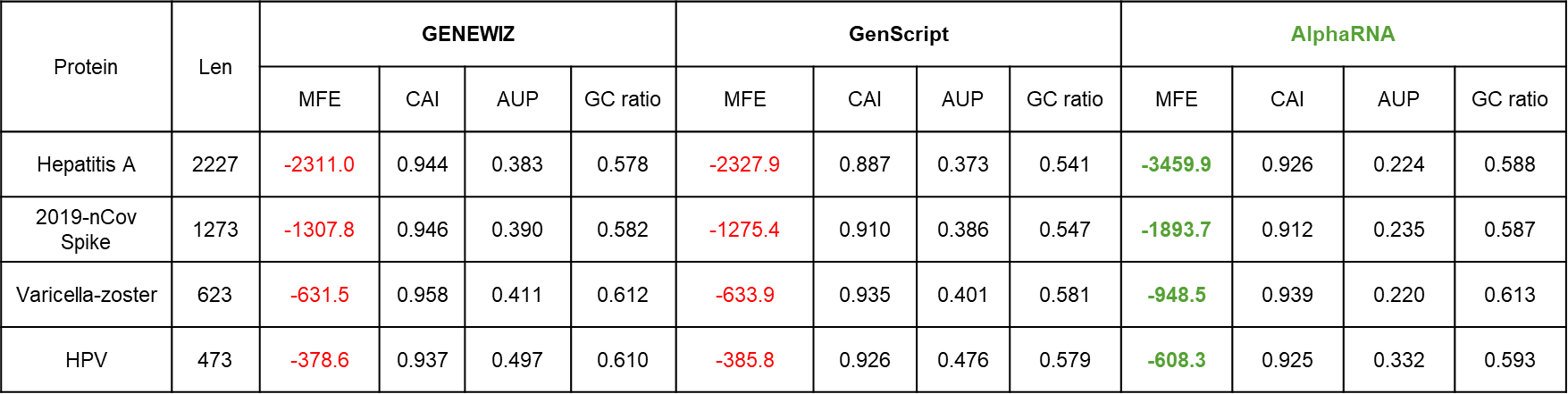
The amino acid sequence of the coding region that needs to be optimized, for example:
MDIDPYKEFGATVELLSFLPSDFFPSVRDLLDTASALYREALESPEHCSPHHTALRQAIL
The restriction enzyme cleavage sites to be limited (avoided in the optimized sequence) can be selected multiple times.
Motif sequences that need to be restricted, multiple can be specified, and new sequences that are not in the list can be manually entered, separated by blanks.
The lambda coefficient of CAI, the larger the positive value, the larger the CAI in the result, you can choose multiple. It can be negative, and the more negative the value is, the greater the reduction in CAI.
The lambda coefficient of GCR, the larger the positive value, the larger the GCR in the result, you can choose multiple. It can be negative, and the more negative the value is, the greater the reduction in GCR.
The output file is result.csv and contains the following information:
| Field Name | Description |
|---|---|
| lambda_cai | Lambda coefficients of CAI |
| lambda_gcr | Lambda coefficients of GCR |
| full_sequence | The optimized sequence |
| CAI | Codon adaption index |
| AUP | Average unpaired probability |
| GCR | The proportion of GC bases |
| MFE Structure | The minimum free energy structure |
| dG(MFE)[kcal/mol] | The value of the minimum free energy |
Extract Fv Sequence 是一个用于从抗体全长序列中提取 Fv 区域(可变区)和 非 Fv 区域 序列的工具。
输入抗体全长序列文件,格式为 FASTA。
指定输出的抗体 Fv 区域序列文件 名称,格式为 FASTA。
工具将输出两个 FASTA 文件:
Fv.fasta:仅包含 Fv 区域序列;nonFv.fasta:包含非 Fv 区域(包括可能存在的 linker)的序列。Extract Fv Sequence is a tool designed to extract the Fv region (variable domain) and non-Fv region sequences from a full-length antibody sequence.
Input full-length antibody sequence file in FASTA format.
Specify the output filename for the Fv region sequence, in FASTA format.
The tool generates two FASTA files:
Fv.fasta: contains only the Fv region sequence;nonFv.fasta: contains the non-Fv region sequence (including any linker regions, if present).
使用动态编程算法预测单链RNA或DNA序列的二级结构,返回单一的RNA最佳结构和最低自由能。
长度为n的序列上的结构由相等长度的括号和点组成的字符串表示。i和j之间的碱基对用“(”在i和“)”在在j位置表示,未配对的碱基用“.”表示。如下为RNA二级结构表示方式。
(((..((((...)))).)))
与之对应的RNA二级结构图为:
RNA序列文件,FASTA格式。
输出文件名称。
输出结果包括:
| 输出文件名称 | 说明 |
|---|---|
| output.txt | RNA序列二级结构的文本文件,其中包括序列、最佳二级结构以及与其对应的最小自由能(kcal/mol)。 |
| SeqN_2D.png | 第N条RNA序列对应的二级结构图 |
The dynamic programming algorithm is used to predict the secondary structure of a single-stranded RNA or DNA sequence, returning the best RNA structure and its minimum free energy.
The structure on a sequence of length n is represented by a string consisting of equal-length parentheses and dots. Base pairs between i and j are represented by “(” at position i and “)” at position j, while unpaired bases are represented by “.”. Below is an example of an RNA secondary structure representation.
(((..((((...)))).)))
The corresponding RNA secondary structure diagram is shown in the image above.
RNA sequence file in FASTA format.
Name of the output file.
The output results include:
| Output File Name | Description |
|---|---|
| output.txt | Text file of the RNA sequence’s secondary structure, including the sequence, best secondary structure, and the corresponding minimum free energy (kcal/mol). |
| SeqN_2D.png | Secondary structure diagram for the Nth RNA sequence |

RNA 3D Structure Prediction是基于Rosetta中的RNA结构建模算法是基于现有RNA晶体结构的短片段(1到3个核苷酸)的组装,其序列与目标RNA的子序列相匹配。RNA片段组装(Fragment Assembly of RNA, FARNA)算法是一个蒙特卡洛过程,由一个低分辨率的基于知识的能量函数指导。然后,这些模型可以在全原子力场下进一步完善,以产生更真实的结构。由此产生的能量也能更好地区分原生构象和非原生构象。该计算方法被称为FARFAR(RNA片段组装与全原子细化)。
从5’到3’的序列。通常用小写字母,但大写字母是可以接受的,并且会被转换。支持多条序列同时生成3D结构。
点括号表示RNA二级结构文件。可以通过模块“RNA Secondary Structure Prediction”获取。
RNA二级结构文件,文本格式,例如:
>a
auauccccauauaucccauauauccccgcgcgucccgcgc
........((((((...))))))....(((((...))))) ( -6.60)
>b
aaauccccauauaucccauauauccccgcgcgucccgcgc
........((((((...))))))....(((((...))))) ( -6.60)
得到RNA结构的PDB文件S_000001.pdb。
RNA 3D Structure Prediction utilizes the RNA structure modeling algorithm in Rosetta, which assembles short fragments (1 to 3 nucleotides) based on existing RNA crystal structures, matching the sequence to a subsequence of the target RNA. The Fragment Assembly of RNA (FARNA) algorithm is a Monte Carlo process guided by a low-resolution, knowledge-based energy function. These models can then be further refined under a full-atom force field to produce more realistic structures. The resulting energy can better distinguish native conformations from non-native conformations. This computational method is known as FARFAR (Fragment Assembly of RNA with Full Atom Refinement).
Sequence(s) from 5’ to 3’. Typically in lowercase letters, but uppercase letters are acceptable and will be converted. Supports generating 3D structures for multiple sequences simultaneously.
RNA secondary structure file in dot-bracket notation. This can be obtained using the “RNA Secondary Structure Prediction” module.
Example RNA secondary structure file in text format:
>a
auauccccauauaucccauauauccccgcgcgucccgcgc
........((((((...))))))....(((((...))))) ( -6.60)
>b
aaauccccauauaucccauauauccccgcgcgucccgcgc
........((((((...))))))....(((((...))))) ( -6.60)
Obtain the PDB file for the RNA structure as S_000001.pdb.
AlphaMHC是唯信计算为解决现有预测方法的已知问题而开发的下一代免疫原性预测算法,采用流行的NLP自然语言处理技术,全新的多模融合深度神经网络架构,整合了近10亿条公开及私有的与免疫原性相关的湿实验数据(包括亲和力数据、NGS数据、质谱数据等)进行训练,成功实现了从序列到临床免疫原性风险的端到端的预测,并通过上百条来自FDA、EMA的临床真实免疫原性数据(包括单/多特异性抗体和重组蛋白等)进行验证,AlphaMHC能够准确区分免疫原性的高低,ROC-AUC达0.87,准确性超过80%(部分测试集高达91%),表现出比现有方法显著更优的预测性能,是已知唯一一个可以得到临床数据验证的算法。
蛋白序列文件,FASTA格式。支持多条链以及多分子模式。
请注意按下面的规则来书写序列名,因为目前免疫原性风险的评分是以整个分子为单位的,链名会影响到程序区分同个分子的多条链,并影响对于分子总的风险评级(risk per molecule),但不影响对链的TCE的识别。
对于多条链的分子,序列名称应写为:分子名.链名,".“之前是分子名,”.“之后是链名,同个分子的不同链,只要”."之前的分子名保持一致就可以了,链名随意,顺序不限。
例如,下面mol1是常见的单抗,mol2是多抗:
>mol1.A
XXXXXXX
>mol1.B
XXXXXXX
>mol2.L1
XXXXXXX
>mol2.H1
XXXXXXX
>mol2.L2
XXXXXXX
>mol2.H2
XXXXXXX
预测HLA等位基因型。
rep:32个代表性等位基因型,适用于一般人群。
all:用于训练的所有非冗余人类等位基因型(1166个)。
一般推荐使用默认的"rep",因为免疫原性的风险评分(risk)是基于rep的代表性HLA来确定的。
导出每个 HLA 等位基因的结合亲和力曲线图,展示了与每条蛋白质链的 N 端到 C 端的所有15肽的结合亲和力。注意:即使“HLA Allotypes”选项设置为全部,也只会绘制代表性 HLA的曲线。
输出结果包括:
| 输出文件名称 | 说明 |
|---|---|
| score_immunogenicity_risk.csv | 该结果展示了预测的每个分子的免疫原性风险(自动将同个分子的多条链的预测的潜在T细胞表位的结果进行汇总后综合评估所得)。 |
| detail_tce_of_chains.csv | 该结果评估可以进行定向改造的HLA呈递表位,以降低免疫原性。 |
| BAProfile_of_mol.chain.png | 不同HLA亚型与每条链的不同位置的亲和力的分布情况,更精细的展示了不同HLA的亲和力的差异。 从左到右的分布图表示从其中一条蛋白质链的N末端移动到C末端的15聚肽窗口的结合亲和力。 即使“HLA同种异型”选项设置为“全部”,也只会包括代表性的HLA等位基因。 |
| Heatmap_of_mol.chain.png | 每个肽与代表性HLA之间结合亲和力的热图。Z-score是pAffinity,值越大(浅色)意味着预测结合越强。 |
其中score_immunogenicity_risk.csv包括信息如下:
| 字段名称 | 说明 |
|---|---|
| Protein_Id | 蛋白序列名称 |
| Risk | 预测的分子整体风险评估,高风险的分子为high,否则为low。 |
| Score | 表位总长度,是整体风险评估的重要依据。 |
| TCE_Sequences | 表位序列 |
其中detail_tce_of_chains.csv包括信息如下:
| 字段名称 | 说明 |
|---|---|
| Sequences | 蛋白序列名称 |
| TCE | 每条链的相对的高风险的T细胞表位 |
| Alleles_Number | 递呈的HLA亚型数 |
| Alleles | 递呈的HLA亚型 |
| Min_Affinity | 亲和力最小值 |
| Median_Affinity | 亲和力中位数 |
| Max_Affinity | 亲和力最大值 |
AlphaMHC is the next-generation immunogenicity prediction algorithm developed by Wecomput using popular NLP natural language processing technology to address known issues with existing prediction methods. It employs a new multi-modal fusion deep neural network architecture and is trained on nearly one billion publicly available and private wet-lab experimental data related to immunogenicity, including affinity data, NGS data, mass spectrometry data, etc. It successfully achieves end-to-end prediction of immunogenicity risk from sequence to clinical application and is validated using hundreds of clinical real-world immunogenicity data from FDA and EMA, including mono/multi-specific antibodies and recombinant proteins. AlphaMHC accurately distinguishes high and low immunogenicity with an ROC-AUC of 0.87 and an accuracy of over 80% (up to 91% on some test sets), demonstrating significantly better predictive performance than existing methods. It is the only known algorithm that has been validated with clinical data.
Protein sequence file in FASTA format.Multiple chains and multi-molecule modes are supported. For multi-molecule mode, the sequence name rule is: molecule name. chain name, for example:
>mol1.A
XXXXXXX
>mol1.B
XXXXXXX
>mol2.A
XXXXXXX
>mol2.B
XXXXXXX
Prediction of HLA allelic types. “rep” is recommended, which is faster.
rep: 32 representative allelic types, applicable to the general population.
all: all non-redundant human allele types used for training (1166).
Export binding affinity curve graphs for each HLA allele, showing the binding affinity of all 15 peptides from the N- to C-terminus for each protein chain. Note: Even if the “HLA Allotypes” option is set to all, curves will only be plotted for representative HLAs.
The output includes:
| Output File Name | Description |
|---|---|
| score_immunogenicity_risk.csv | The result displays the immunogenicity risk for each predicted molecule (which is obtained by aggregating the predicted potential T cell epitopes from multiple chains of the same molecule and evaluating the overall risk). |
| detail_tce_of_chains.csv | The results evaluated HLA presentation epitopes that could be targeted for engineering to reduce immunogenicity. |
| BAProfile_of_mol.chain.png | The distribution profile of the binding affinity between each chain and the 32 representative HLAs. The profile from left to right represents the binding affinity of a 15-mer pepetide window moving from the N terminus to C terminus of one of the protein chain. PS. only representative HLA alleles will be included even if the “HLA allotypes” option is set to “all”. |
| Heatmap_of_mol.chain.png | The heat map of the binding affinity between each peptide and the representative HLAs. The Z-score is pAffinity, greater value (light color) means stronger binding by prediction. |
score_immunogenicity_risk.csv contains the following information:
| Field Name | Description |
|---|---|
| Protein_Id | Protein sequence name |
| Risk | The overall risk assessment for the predicted molecule, with “high” indicating high-risk molecules and “low” indicating low-risk molecules. |
| Score | The total length of the epitopes, which is an important basis for overall risk assessment. |
| TCE_Sequences | The epitope sequences |
detail_tce_of_chains.csv contains the following information:
| Field Name | Description |
|---|---|
| Sequences | Protein sequence name |
| TCE | The relative high risk T cell epitope of each strand. |
| Alleles_Number | Number of HLA subtypes presented |
| Alleles | The HLA subtypes presented |
| Min_Affinity | Affinity minimum |
| Median_Affinity | Median affinity |
| Max_Affinity | Affinity maximum |

基于知名的DNAWorks算法对氨基酸或DNA序列进行密码子优化(基于PCR的基因合成的自动寡核苷酸设计)。
整个基因组序列的可用性极大地增加了蛋白质靶标的数量,其中许多需要在原始DNA来源以外的细胞中过度表达。合成基因可以针对表达进行优化,并构建为易于突变操作而无需考虑亲本基因组。然而,合成基因的设计和构建,尤其是那些编码大蛋白质的基因,可能是一个缓慢、困难和令人困惑的过程。该模块通过基于PCR的方法自动设计用于基因合成的寡核苷酸。

蛋白或者核酸的序列文件,FASTA格式。
序列类型,蛋白或者核酸。
几种常用生物的密码子频率基于每个密码子在相应生物基因组的蛋白质编码区中出现的次数。大肠杆菌有两种选项:基于所有基因的标准频率(E. coli),或在指数增长期间以高水平表达的 II 类基因频率(ecoli2),通常建议用后者。
退火温度参数为一组合成寡核苷酸设定了理想的退火温度。 可接受的退火温度范围在 58 至 70°C 之间。
寡核苷酸长度参数限制了一组合成寡核苷酸中的任何一个可以达到的核苷酸长度。可接受的寡核苷酸长度范围在 30 到 999 nt 之间。
密码子频率阈值参数设置:密码子用于反向翻译蛋白质序列到DNA的截断值。
寡核苷酸的浓度。寡核苷酸必须在100 uM (1E-4 M)和1 nM (1E-9 M)之间。
一价阳离子(Na+,K+)的浓度。单价阳离子必须在10到1000mM之间。
镁离子的浓度。镁离子浓度必须在0到200mM之间。
执行中生成的寡核苷酸的数量,每个作业的最大运行次数为999次。
检查是否为热力学平衡由内而外合成法 (thermodynamically balanced inside-out, TBIO)输出模式。
要求被排除在合成基因的蛋白质编码区之外的位点,每个位点之间用逗号隔开,例如Aatll,Acc65I。
支持非简并位点共117种:
AatII,Acc65I,AclI,AcuI,AfeI,AflII,AgeI,AlwI,ApaI,ApaLI,AscI,AseI,AsiSI,AvrII,BamHI,BbsI,BbvCI,BbvI,BccI,BceAI,BciVI,BclI,BfrBI,BfuAI,BglII,BmgBI,BmrI,BmtI,BpmI,BpuEI,BsaI,BseRI,BseYI,BsgI,BsiWI,BsmAI,BsmBI,BsmFI,BsmI,BspCNI,BspDI,BspEI,BspHI,BspMI,BsrBI,BsrDI,BsrGI,BsrI,BssHII,BssSI,BstBI,BstZ17I,BtgZI,BtsI,ClaI,DraI,EagI,EarI,EciI,EcoRI,EcoRV,FauI,FokI,FseI,FspI,HgaI,HindIII,HpaI,HphI,KasI,KpnI,MboII,MfeI,MluI,MlyI,MscI,NaeI,NarI,NcoI,NdeI,NgoMIV,NheI,NotI,NruI,NsiI,PacI,PaeR7I,PciI,PleI,PmeI,PmlI,PsiI,PspOMI,PstI,PvuI,PvuII,SacI,SacII,SalI,SapI,SbfI,ScaI,SfaNI,SfoI,SmaI,SnaBI,SpeI,SphI,SspI,StuI,SwaI,TliI,TspRI,XbaI,XhoI,XmaI,ZraI
支持简并位点共62种:
AccI,AflIII,AhdI,AleI,AlwNI,ApoI,AvaI,BanI,BanII,BcgI,BglI,BlpI,Bme1580I,Bpu10I,BsaAI,BsaBI,BsaHI,BsaJI,BsaWI,BsaXI,BsiEI,BsiHKAI,BslI,BsoBI,Bsp1286I,BsrFI,BstAPI,BstEII,BstF5I,BstXI,BstYI,Bsu36I,BtgI,Cac8I,DraIII,DrdI,EaeI,EcoNI,EcoO109I,HaeII,HincII,Hpy188III,MmeI,MslI,MspA1I,MwoI,NlaIV,NspI,PflFI,PflMI,PpuMI,PshAI,RsrII,SexAI,SfcI,SfiI,SgrAI,SmlI,StyI,Tth111I,XcmI,XmnI
自定义被排除在合成基因的蛋白质编码区之外的位点,自定义位点格式必须包含名称和序列,名称和序列之间用空格隔开,多个位点时用逗号隔开,例如:Aatll GACGTC,Acc65I GGTACC。
输出结果文件的名称。
输出结果文件为result.txt,包含优化后的密码子序列以及序列相关信息。
Codon optimization can be used for optimizing codons (i.e., the genetic code) for the automated oligonucleotide design of gene synthesis based on PCR. The availability of whole genome sequences has greatly increased the number of protein targets, many of which need to be overexpressed in cells outside of their native DNA source. Synthetic genes can be optimized for expression and constructed to be easily mutagenized without consideration for the parental genome. However, designing and constructing synthetic genes, particularly those encoding large proteins, can be a slow, difficult, and confusing process. This module automatically designs oligonucleotides for gene synthesis using a PCR-based approach.
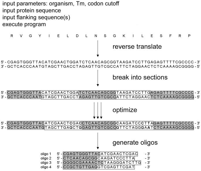
Protein or nucleotide sequences in FASTA format
Sequence files of proteins or nucleic acids
The codon frequencies of several commonly used organisms are based on the number of times each codon appears in the protein-coding regions of the respective organism’s genome. For Escherichia coli, there are two options: the standard frequency based on all genes (E. coli), or the frequency of Class II genes expressed at high levels during exponential growth (ecoli2), which is usually recommended to be used.
The annealing temperature parameter sets the ideal annealing temperature for a set of synthetic oligonucleotides. Acceptable annealing temperatures range from 58 to 70°C.
The oligonucleotide length parameter limits the achievable nucleotide length of any one of a set of synthetic oligonucleotides. Acceptable oligonucleotide lengths range from 30 to 999 nt.
Codon Frequency Threshold Parameter Settings: Codon cutoff value for backtranslation of protein sequences to DNA.
Concentration of oligonucleotides. Oligonucleotides must be between 100 uM (1E-4 M) and 1 nM (1E-9 M).
Concentration of monovalent cations (Na+, K+). Monovalent cations must be between 10 and 1000 mM.
concentration of magnesium ions. Magnesium ion concentration must be between 0 and 200mM.
The number of oligos generated in an execution, with a maximum of 999 runs per job.
Check if it is thermodynamically balanced inside-out (TBIO) output mode.
Sites required to be excluded from the protein coding region of the synthetic gene, separated by commas between each site, example: Aatll,Acc65I.
Support a total of 117 non-degenerate sites:
AatII,Acc65I,AclI,AcuI,AfeI,AflII,AgeI,AlwI,ApaI,ApaLI,AscI,AseI,AsiSI,AvrII,BamHI,BbsI,BbvCI,BbvI,BccI,BceAI,BciVI,BclI,BfrBI,BfuAI,BglII,BmgBI,BmrI,BmtI,BpmI,BpuEI,BsaI,BseRI,BseYI,BsgI,BsiWI,BsmAI,BsmBI,BsmFI,BsmI,BspCNI,BspDI,BspEI,BspHI,BspMI,BsrBI,BsrDI,BsrGI,BsrI,BssHII,BssSI,BstBI,BstZ17I,BtgZI,BtsI,ClaI,DraI,EagI,EarI,EciI,EcoRI,EcoRV,FauI,FokI,FseI,FspI,HgaI,HindIII,HpaI,HphI,KasI,KpnI,MboII,MfeI,MluI,MlyI,MscI,NaeI,NarI,NcoI,NdeI,NgoMIV,NheI,NotI,NruI,NsiI,PacI,PaeR7I,PciI,PleI,PmeI,PmlI,PsiI,PspOMI,PstI,PvuI,PvuII,SacI,SacII,SalI,SapI,SbfI,ScaI,SfaNI,SfoI,SmaI,SnaBI,SpeI,SphI,SspI,StuI,SwaI,TliI,TspRI,XbaI,XhoI,XmaI,ZraI
Support a total of 62 degenerate sites:
AccI,AflIII,AhdI,AleI,AlwNI,ApoI,AvaI,BanI,BanII,BcgI,BglI,BlpI,Bme1580I,Bpu10I,BsaAI,BsaBI,BsaHI,BsaJI,BsaWI,BsaXI,BsiEI,BsiHKAI,BslI,BsoBI,Bsp1286I,BsrFI,BstAPI,BstEII,BstF5I,BstXI,BstYI,Bsu36I,BtgI,Cac8I,DraIII,DrdI,EaeI,EcoNI,EcoO109I,HaeII,HincII,Hpy188III,MmeI,MslI,MspA1I,MwoI,NlaIV,NspI,PflFI,PflMI,PpuMI,PshAI,RsrII,SexAI,SfcI,SfiI,SgrAI,SmlI,StyI,Tth111I,XcmI,XmnI
Custom sites that to be excluded from the protein coding region(s) of the synthetic gene. The custom site format must contain the name and sequence, separated by a space between the name and sequence, and separated by a comma when there are multiple sites. Example: Aatll GACGTC,Acc65I GGTACC.
Specify output file name
The output file is result.txt, which contains the optimized codon sequence and sequence-related information.

PDB Mutation是用于突变PDB格式的蛋白质结构并返回突变后的结构。
蛋白的结构文件,PDB格式
为后续突变文件中的残基索引设置类别。有两种选择:UID或者POS
UID表示PDB文件中自带的残基编号,该编号可能存在间断不连续,不从1开始等情况;
POS表示位置编号或自然顺序编号,从1开始按顺序进行编号。默认为POS。
突突变文本文件,包含突变信息,格式如下:
KA100N,KA101T
KA100T
KA100BT
每个突变定义为:
第一字母代表的是原始残基,第二个字母代表PDB文件中待突变残基所在的链名,后面的数字代表残基位置编号(编号类型是POS还是UID,在上述参数Index Type中定义,默认为POS),最后一个字母代表突变后的残基。如:KA100N表示A链中位置编号(POS)100的残基K,突变为N。
KA100BT,表示A链中UID编号为100B的残基K,突变为T。输出结果包括:
| 输出文件名称 | 说明 |
|---|---|
| mutations.tar.gz | 所有突变体PDB结构的压缩包文件 |
| 第一组突变对应的PDB结构 | 如:KA100N_KA101T.pdb |
PDB Mutation is a tool used to mutate protein structures in PDB format and return the mutated structures.
Structure file of the protein in PDB format.
This parameter sets the residue index convention used in the mutation file. Two options are available: UID or POS.
A plain-text file that lists the desired mutations. Format:
KA100N,KA101T
KA100T
KA100BT
Each mutation is defined as follows:
Index Type parameter above; the default is POS).For example, KA100N means that residue K at position 100 (POS) in chain A is mutated to N.
Each line may contain a set of mutations, separated by commas. All mutations in the same line are applied together to generate one new structure file.
Each line corresponds to one newly generated structure file.
UID indexing supports insertion codes. For example, KA100BT means that residue K with UID 100B in chain A is mutated to T.
The output results include:
| Output File Name | Description |
|---|---|
| mutations.tar.gz | Compressed file containing all mutated PDB structures |
| The PDB structure that corresponds to the first set of mutations | such as: KA100N_KA101T.pdb |
通过解析美国(https://patentcenter.uspto.gov/)和国际(https://patentscope2.wipo.int/search/en/search.jsf)专利附带的序列清单(Sequence Listing)文件,里面存储了专利权利要求的序列,但是人工很难读取,该模块可以从中一次性批量提取专利中所有具有正式编号(SEQ ID NO.)的序列。
1. Sequence Listing文件下载
序列清单(Sequence Listing)文件内容示例:

用法:
(1)从专利网站搜索专利:
(2)在专利的页面中找到Sequence Listing文件并下载。
从WIPO网站下载
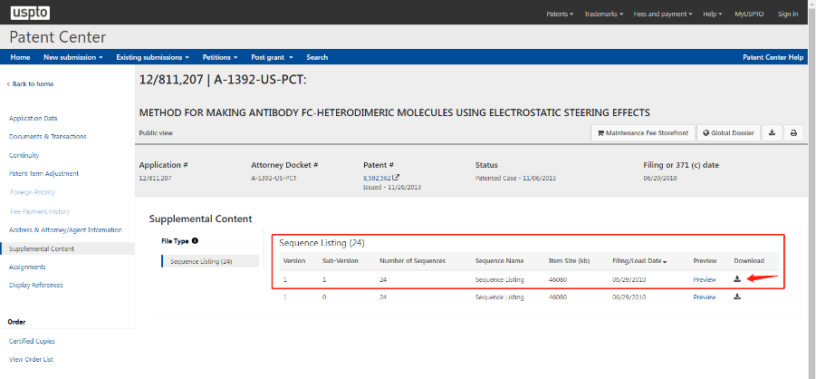
从USPTO网站下载
(3)使用该模块,提交下载到的文件即可。
2. Image(OCR)
将图片中的蛋白质序列转换为3个字母编码或1个字母编码的序列。
注意:截图时请务必省略标题,类似下图。
专利文件,TXT或者XML格式。
输出结果包括:
| 输出文件名称 | 说明 |
|---|---|
| seq_list.csv | 记录所有序列信息的csv文件 |
| seq_list.fasta | 记录所有序列信息的fasta文件 |
其中seq_list.csv包括信息如下:
| 字段名称 | 说明 |
|---|---|
| idx | 序列编号 |
| type | 序列类型,DNA/蛋白 |
| sequence | 序列信息 |
专利图片文件,PNG或者JPG格式
区分蛋白质序列“三字母”和“单字母”的输入,该选项用于指定识别模式:3L 表示 3-letter,1L 表示 1-letter。
输出文件名称,默认为result.fasta
输出结果包括:
| 输出文件名称 | 说明 |
|---|---|
| result.fasta | 专利图片转换成一个字母序列的FASTA文件 |
| result.txt | 包含图片文件的字符,转换成一个字母和三个字母的序列 |
By parsing the sequence listing files attached to U.S. (https://patentcenter.uspto.gov/) and international (https://patentscope2.wipo.int/search/en/search.jsf) patents, which store the sequences claimed in patents, it is difficult for humans to read them. This module can extract all sequences with official numbers (SEQ ID NO.) from the patents in bulk.
1. Sequence Listing File Download
Example content of a Sequence Listing file:
Usage:
(1) Search for patents on patent websites:
2. Image(OCR)
Image(OCR) is for converting protein sequences from images into three-letter or one-letter coded sequences.
Note: When taking screenshots, please be sure to omit the headers, similar to the image below.
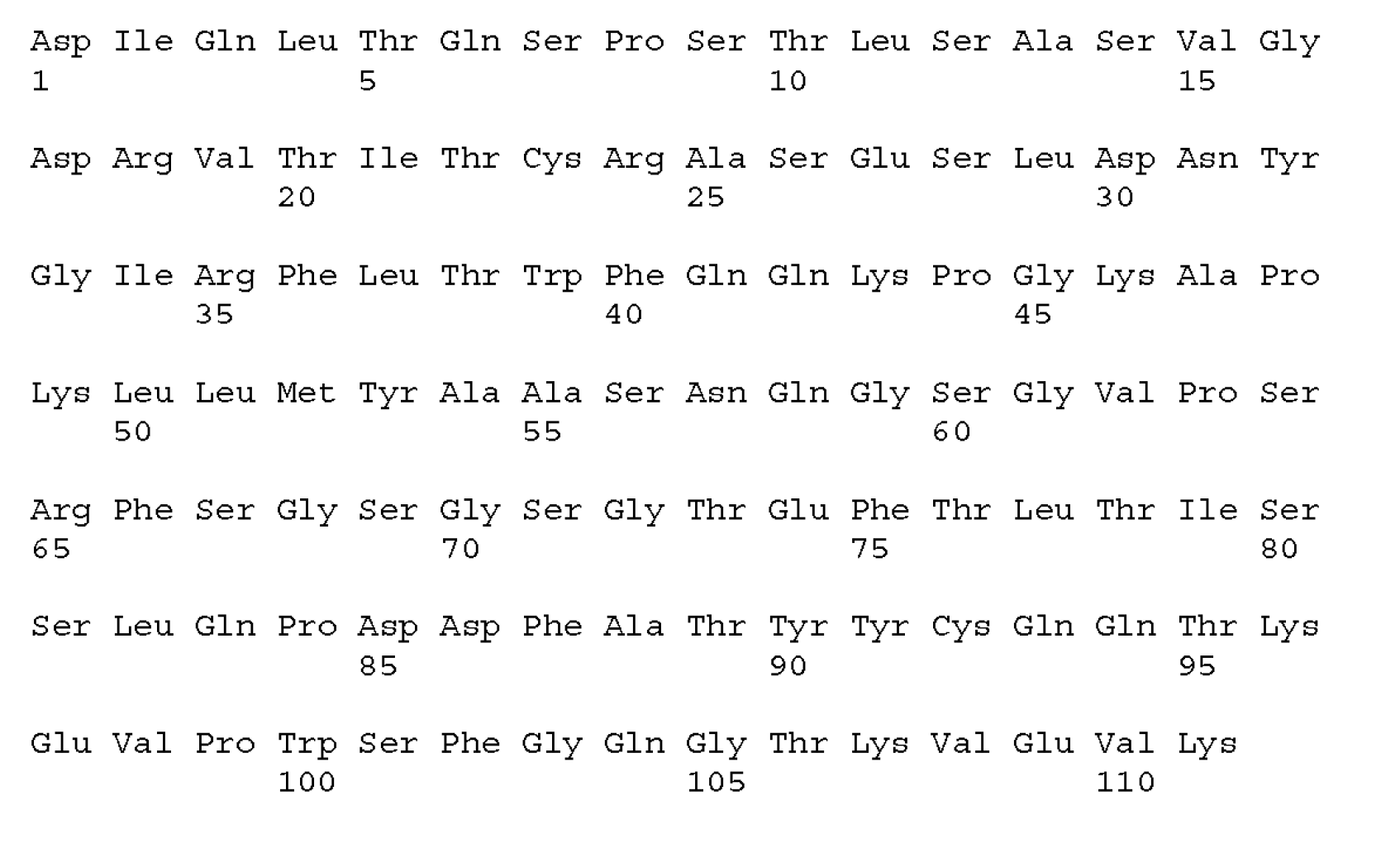
Patent file in TXT or XML format.
The output includes:
| Output File Name | Description |
|---|---|
| seq_list.csv | CSV file recording all sequence information |
| seq_list.fasta | FASTA file recording all sequence information |
The seq_list.csv includes the following information:
| Field Name | Description |
|---|---|
| idx | Sequence number |
| type | Sequence type, DNA/protein |
| sequence | Sequence information |
Patent image file in PNG or JPG format
Distinguishes between protein sequence inputs in three-letter and one-letter formats. This option specifies the recognition mode: 3L for three-letter and 1L for one-letter.
Output file name, default is result.fasta
The output includes:
| Output File Name | Description |
|---|---|
| result.fasta | FASTA file of one-letter sequences converted from patent images |
| result.txt | Characters from image files converted into one-letter and three-letter sequences |
基于TCGA和GTEx等数据,检索指定基因在肿瘤和正常组织的表达情况,统计并绘制肿瘤细胞、肿瘤组织、正常组织等的基因表达差异,帮助药物靶点选择、研发立项和决策。
基因名称,输入的基因名须对应HGNC(https://www.genenames.org/)的"Approved Symbol"。例如:在HGNC搜索“PD-1”,得知“approved symbol”为“PDCD1”,后者“PDCD1”是该程序需要的输入。
注意:HGNC网站会更新基因命名。如果输入的Approved Symbol报错,可尝试使用Previous Symbol。例如,“AARS1” 基因可输入为 “AARS”。
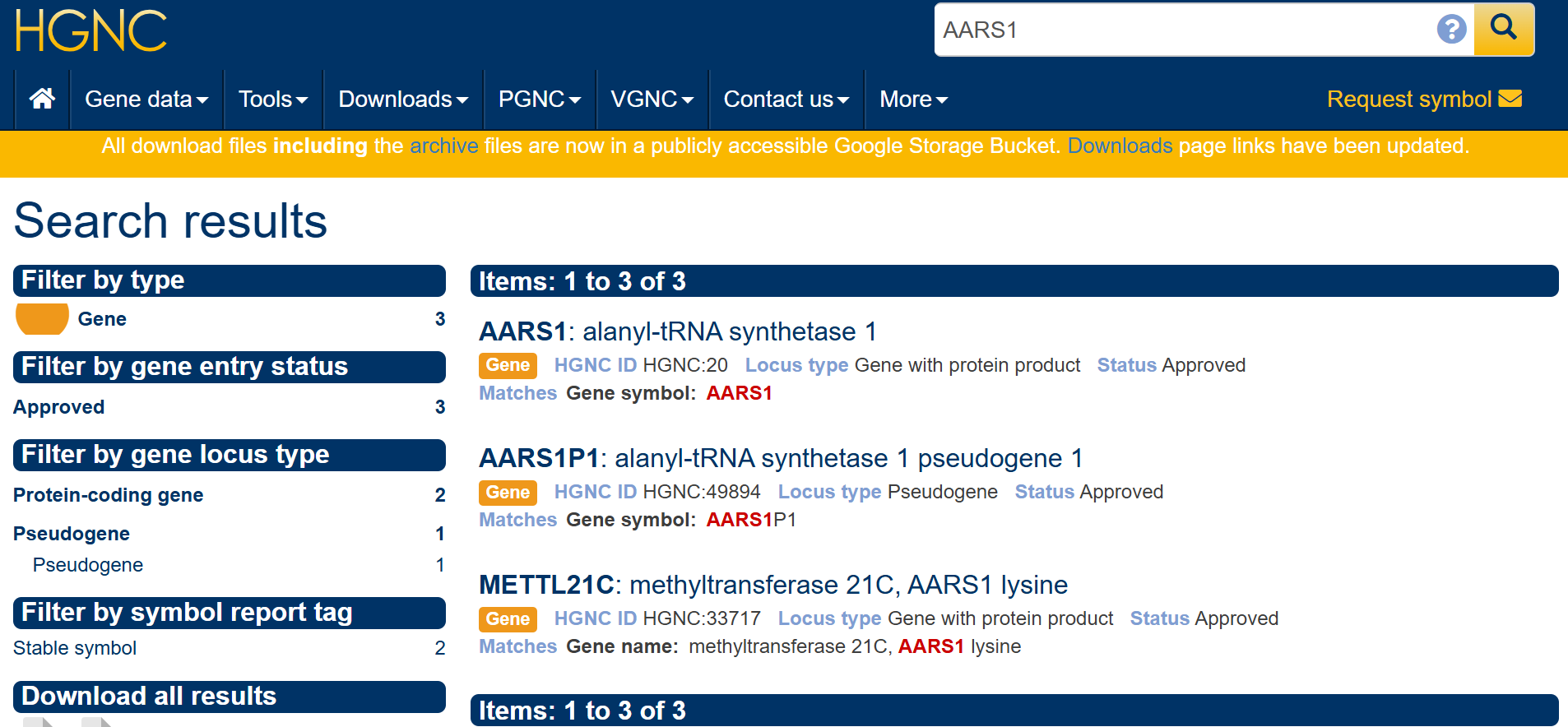
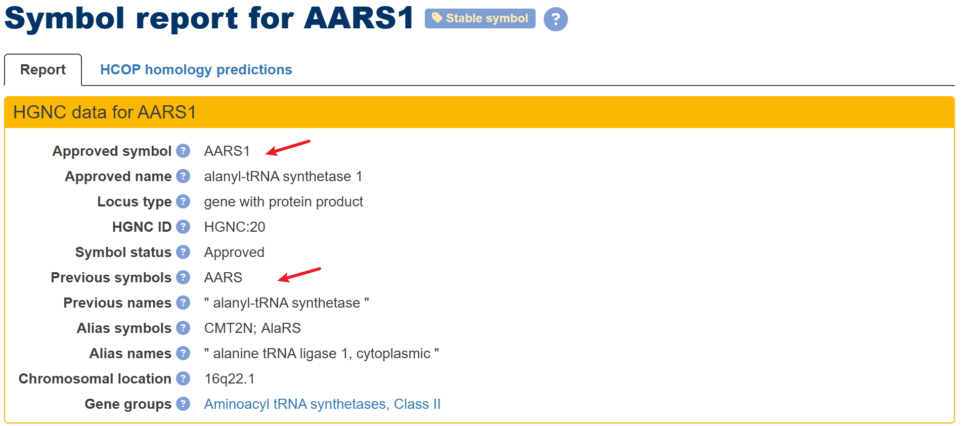
输出结果包括:
| 输出文件名称 | 说明 |
|---|---|
| tcga_expression.jpeg | 不同疾病中该基因分别在肿瘤、正常、癌旁组织的表达量分布。 |
| tcga_tissue_expression.jpeg | 不同组织中该基因分别在肿瘤、正常、癌旁组织的表达量分布。 |
Plot gene expression in normal and tumor tissues, based on databases TCGA and GTEx. It retrieves the expression of specified genes in tumors and normal tissues, counts and maps the gene expression differences of tumor cells, tumor tissues, and normal tissues, etc., to help drug target selection and decision-making.
The entered gene name must correspond to the “Approved Symbol” of HGNC (https://www.genenames.org/). For example: search for “PD-1” in HGNC, and know that “approved symbol” is “PDCD1”, and the latter “PDCD1” is the input required by the program.
Note: Gene names on the HGNC website are subject to updates. If the Approved Symbol returns an error, try using a Previous Symbol. For example, the gene “AARS1” can be entered as “AARS”.
The output includes:
| Output File Name | Description |
|---|---|
| tcga_expression.jpeg | The program will return the expression distribution of the gene in tumor, normal, and adjacent tissues in different disease. |
| tcga_tissue_expression.jpeg | The program will return the expression distribution of the gene in tumor, normal, and adjacent tissues in different tissues. |
Multiple Sequence Alignment 是多重序列比对模块,用于进化分析,绘制进化树,帮助对候选序列进行聚类、分析多样性等。
蛋白序列文件,FASTA格式。
蛋白序列文件,FASTA格式。
抗体编号方法,支持imgt,kabat,chothia
输出抗体整体序列一致性文件名称,CSV格式
输出抗体CDR序列一致性文件名称,CSV格式
输出抗体序列一致性热图,HTML格式
输出结果包括:
| 输出文件名称 | 说明 |
|---|---|
| alignment.fasta | 多重序列进行比对后的FASTA文件 |
| alignment.png | 多重序列进行比对后的PNG文件 |
| newick.txt | 多重序列进行多样性分析的结果文件 |
| tree.png | 多重序列进化树图片 |
| out/full_identity.csv | 针对抗体方法下,抗体整体序列一致性CSV文件 |
| out/cdr_identity.csv | 针对抗体方法下,抗体CDR序列一致性CSV文件 |
| out/identity_heatmap.html | 针对抗体方法下,抗体序列一致性热图HTML文件 |
Multiple Sequence Alignment is a module for aligning multiple sequences, used for evolutionary analysis, drawing evolutionary trees, and aiding in clustering and analyzing diversity of candidate sequences.
Protein sequence file in FASTA format
Antibody sequence file in FASTA format.
Antibody numbering scheme, supporting imgt, kabat, and chothia
Export pairwise full identity matrix as CSV
Export pairwise antibody CDR identity matrix as CSV
Ouput antibody sequence identity heatmap in HTML format
The output includes:
| Output File Name | Description |
|---|---|
| alignment.fasta | FASTA file after aligning multiple sequences |
| alignment.png | PNG file after aligning multiple sequences |
| newick.txt | Evolutionary analysis result of multiple sequence |
| tree.png | Evolutionary trees picture of multiple sequence |
| out/full_identity.csv | only for antibody, pairwise full identity matrix CSV file |
| out/cdr_identity.csv | only for antibody, pairwise antibody CDR identity matrix CSV file |
| out/identity_heatmap.html | only for antibody, antibody sequence identity heatmap in HTML format |
Structural Alignment是对两个蛋白质的三维结构进行叠合的工具。使用BLOSUM62矩阵和Needleman-Wunsch算法在两个序列之间执行全局配对比对,返回叠合后的蛋白结构,同时输出RMSD值。
参考蛋白的结构文件,PDB格式
需要叠合蛋白的结构文件,PDB格式
指定参考蛋白的链名,默认是A链
指定需要叠合蛋白的链名,默认是A链
指定输出叠合后的结构文件,PDB格式
输出结果包括:
| 输出文件名称 | 说明 |
|---|---|
| result.csv | 参考蛋白与样本蛋白之间的RMSD值记录文件 |
| alignment_renumbering_pred.pdb | 叠合后的结构文件 |
其中result.csv包含如下信息:
| 字段名称 | 说明 |
|---|---|
| Reference | 参考蛋白构象 |
| Sample | 需要叠合的蛋白构象 |
| RMSD | 叠合后的RMSD值 |
Structural Alignment is a tool for overlaying the 3D structures of two proteins. It performs a global pairwise alignment between two sequences using the BLOSUM62 matrix and the Needleman-Wunsch algorithm, returning the aligned protein structures and outputting the RMSD value.
Structure file of the reference protein in PDB format.
Structure file of the protein to be aligned in PDB format.
Specify the chain name of the reference protein, default is chain A.
Specify the chain name of the protein to be aligned, default is chain A.
Specify the output structure file after alignment in PDB format.
The output results include:
| Output File Name | Description |
|---|---|
| result.csv | RMSD value record file between the reference protein and the sample protein |
| alignment_renumbering_pred.pdb | Aligned structure file |
The result.csv file contains the following information:
| Field Name | Description |
|---|---|
| Reference | Conformation of the reference protein |
| Sample | Conformation of the protein to be aligned |
| RMSD | RMSD value after alignment |
PDB Insertion Removal模块用于去掉抗体PDB文件中的插入序列,因为某些计算工具不支持PDB中的插入序列。比如,20A改成20。
抗体结构文件,PDB格式。
得到去掉抗体中的插入序列的PDB文件prepared_insert.pdb。
The PDB Insertion Removal module is used to remove insertion sequences from antibody PDB files because some computational tools do not support insertion sequences in PDB files. For example, changing 20A to 20.
Antibody structure file in PDB format.
Obtain the PDB file prepared_insert.pdb with the insertion sequences removed from the antibody.
该模块用于预测蛋白质结构中的聚集倾向和蛋白质溶解度,通过考虑序列和结构来预测蛋白质中易聚集的位点,这对于球状蛋白质特别有用,其中容易聚集的位点可能埋藏在天然结构内并且序列不连续。通过考虑天然氨基酸的实验聚集倾向尺度,该方法可以准确预测蛋白质聚集倾向,也可用于预测构象紊乱中家族性突变的致病作用。任何已知或预测的蛋白质结构都是适用的,它具备其他基于序列的算法未考虑的特性,例如蛋白质动态波动和蛋白质序列中距离较远的残基的空间聚类,这对于从初始折叠状态准确预测蛋白质聚集非常重要。
底层算法Aggrescan3D(A3D)旨在预测蛋白质在其折叠状态下的聚集倾向。为了实现这个目标,A3D使用蛋白质的三维结构作为输入,这些结构可以通过X射线衍射、溶液NMR或建模方法得到,并以pdb格式表示。在分析之前,这些结构会经过能量最小化处理。该方法利用了实验得出的天然氨基酸内在聚集倾向尺度,并将这个尺度应用于蛋白质的三维结构中。在A3D方法中,结构中每个特定氨基酸的内在聚集倾向会受到其特定的结构环境的调节。聚集倾向是通过以每个残基Cα碳为中心的球形区域计算得出的。这为结构中每个氨基酸提供了一个独特的经过结构修正的聚集值(A3D分数),其公式如下:

其中:Aggi是球心处残基的内在聚集倾向;RSAi是其相对于溶剂暴露的表面积;Agge是包括在球体中的每个额外残基的内在聚集倾向,RSAe是其相对于溶剂暴露的表面积,dist是到中心残基i的距离。
蛋白质结构文件(PDB 格式)。
支持上传包含多个结构文件的压缩包进行批量处理,包括 .zip、.tar、.tar.gz、.tgz、.tar.bz2、.tbz2、.tar.xz、.txz格式
注意
输出结果包括:
| 名称 | 说明 |
|---|---|
| Aggregation Score (result_A3D.csv) | 蛋白结构中每个氨基酸聚集倾向和蛋白质溶解度的打分文件 |
| Structure (output.pdb) | 根据聚集倾向和蛋白质溶解度得到的结构文件,在PDB文件温度因子一栏填入计算得到的聚集度和溶解度数值 |
| all_results_AggS.tar.gz | 当输入为压缩包格式并包含多个结构文件时,系统会将每个结构对应的计算结果汇总并打包为该压缩文件输出。 |
| result_A.png | A链中每个氨基酸对应的聚集度和溶解度打分值的png格式图片 |
| result_A.svg | A链中每个氨基酸对应的聚集度和溶解度打分值的svg格式图片 |
其中result_A3D.csv包括信息如下:
| 字段名称 | 说明 |
|---|---|
| protein | 氨基酸残基折叠 |
| chain | 蛋白链名称 |
| residue | 氨基酸索引(PDB文件中) |
| residue_name | 氨基酸名称缩写(PDB文件中) |
| score | 聚集度和溶解度打分值,该数值为正代表氨基酸促进聚集,为负代表氨基酸促进溶解。 |
This module is used to predict the aggregation propensity and protein solubility in protein structures. By considering both sequence and structure, it predicts sites in proteins that are prone to aggregation, which is particularly useful for globular proteins where aggregation-prone sites may be buried within the native structure and not contiguous in sequence. By considering experimentally derived aggregation propensity scales of natural amino acids, this method accurately predicts protein aggregation propensity and can be used to predict the pathogenic effects of familial mutations in conformational disorders. Any known or predicted protein structure is applicable. It incorporates features not considered by other sequence-based algorithms, such as protein dynamic fluctuations and spatial clustering of residues that are distant in the protein sequence, which is crucial for accurately predicting protein aggregation from the initial folding state.
The underlying algorithm, Aggrescan3D (A3D), aims to predict the aggregation propensity of proteins in their folded states. To achieve this, A3D uses the protein’s 3D structure as input, which can be obtained through X-ray crystallography, solution NMR, or modeling methods, and is represented in PDB format. These structures undergo energy minimization before analysis. The method utilizes experimentally determined intrinsic aggregation propensity scales of natural amino acids and applies this scale to the protein’s 3D structure. In the A3D method, the intrinsic aggregation propensity of each specific amino acid in the structure is modulated by its specific structural environment. The aggregation propensity is calculated within a spherical region centered on the Cα carbon of each residue. This provides a unique, structurally corrected aggregation value (A3D score) for each amino acid in the structure.The calculation formula is as follows:
Where:
The system accepts protein structure files in PDB format. For batch processing, you may upload a compressed archive containing multiple structure files. Supported archive formats include .zip, .tar, .tar.gz, .tgz, .tar.bz2, .tbz2, .tar.xz, and .txz.
Notes
The output results include:
| Name | Description |
|---|---|
| Aggregation Score (result_A3D.csv) | A scoring file for the aggregation propensity and protein solubility of each amino acid in the protein structure. |
| Structure (output.pdb) | Structure file obtained based on the aggregation propensity and protein solubility, with the calculated aggregation and solubility values filled in the temperature factor column of the PDB file. |
| all_results_AggS.tar.gz | When the input is provided as a compressed archive containing multiple structure files, the calculation results for each structure are collected and packaged into this archive for download. |
| result_A.png | A PNG format image showing the aggregation and solubility scores for each amino acid in chain A. |
| result_A.svg | An SVG format image showing the aggregation and solubility scores for each amino acid in chain A. |
The result_A3D.csv file includes the following information:
| Field Name | Description |
|---|---|
| protein | Fold of the amino acid residue. |
| chain | Protein chain name. |
| residue | Amino acid index in the PDB file. |
| residue_name | Amino acid name abbreviation in the PDB file. |
| score | Aggregation and solubility score, where a positive value indicates promotion of aggregation and a negative value indicates promotion of solubility. |
Sequence Mutagenesis (Saturated)是用于枚举蛋白质序列指定位置饱和突变的所有可能性,生成所有对应突变的文本文件和突变体序列文件。
蛋白序列文件,FASTA格式。
突变位置,多个位置可以用逗号(,)隔开。
指定输出突变后的序列文件的名称,FASTA格式。
包含突变信息的文本文件的名称。
指定链名,生成带有链名的突变信息。
输出结果包括:
| 输出文件名称 | 说明 |
|---|---|
| mutated_seqs.fasta | 突变后的序列文件 |
| individual.txt | 突变文件信息,包含链信息 |
| mutated_polict.txt | 突变文件信息,不包含链信息 |
Sequence Mutagenesis (Saturated) is used to enumerate all possibilities of saturated mutations at specified positions in a protein sequence, generating text files with all corresponding mutations and mutated sequence files.
Protein sequence file in FASTA format.
Mutation locations, multiple positions can be separated by commas (,).
Specify the name of the output file containing the mutated sequence in FASTA format.
Name of the text file containing mutation information.
Specify the chain name to generate mutation information with chain names.
The output results include:
| Output File Name | Description |
|---|---|
| mutated_seqs.fasta | Mutated sequence file after mutation. |
| individual.txt | Mutation file information with chain information. |
| mutated_polict.txt | Mutation file information without chain information. |
对复合物界面区域进行单点或者多点的虚拟饱和突变,从而获得不同格式的突变文件以及突变后的Fasta文件。这为后续复合物之间的亲和力以及对突变体之间的结合自由能计算提供基础。
蛋白结构文件,PDB格式。
突变位点文件,JSON格式,一般由Complex Interface Analysis模块生成的json文件。
指定链名。
指定输出突变后的序列文件的名称。
指定输出突变文件的名称,不包含链信息。
指定输出突变文件的名称,包含指定链信息。
突变模式:
输出结果包括:
| 输出文件名称 | 说明 |
|---|---|
| mutated_policy.txt | 突变文件信息,不包含链信息 |
| mutated_policy_with_chain.txt | 突变文件信息,包含链信息 |
| output_mutated_seqs.fasta | 突变后的序列文件 |
Virtual saturation mutagenesis is performed on single or multiple points in the interface region of a complex to generate mutation files in different formats and mutated Fasta files. This provides a basis for calculating the affinity between complexes and the binding free energy between mutants.
Protein structure file in PDB format.
Mutation site file in JSON format, typically generated by the Complex Interface Analysis module.
Specify the chain name.
Specify the name of the output file containing the mutated sequence.
Specify the name of the output mutation file without chain information.
Specify the name of the output mutation file with specified chain information.
Mutation mode:
The output results include:
| Output File Name | Description |
|---|---|
| mutated_policy.txt | Mutation file information without chain information. |
| mutated_policy_with_chain.txt | Mutation file information with chain information. |
| output_mutated_seqs.fasta | Mutated sequence file after mutation. |
Protein BLAST是蛋白Blast数据库,该数据库序列整合了GenPept、Swissprot、PIR、PDF、PDB、RefSeq等序列数据库。
蛋白序列文件,FASTA格式。
指定序列比对数据库类型:蛋白,抗体,或者CDR区域。
nr:蛋白Blast数据库。
oas:Observed Antibody Space,抗体Blast数据库。
cdr:CDR区域数据库,专利保护抗体数据库 。
输出结果文件为alignment.fasta,是系列对齐后的FASTA文件,可在WeSeq中查看。
Protein BLAST is a protein Blast database that integrates sequences from databases such as GenPept, Swissprot, PIR, PDF, PDB, RefSeq, and others.
Protein sequence file in FASTA format.
Specifies the sequence alignment database type: protein, antibody, or CDR region.
nr: Protein BLAST database.
oas: Observed Antibody Space, an antibody BLAST database.
cdr: CDR region database, a patent-protected antibody database.
The output result file is alignment.fasta, which is a FASTA file of the aligned sequences that can be viewed in WeSeq.

Sequence Mutagenesis (Directed) for Ab是根据模板抗体序列和描述突变的突变文件(json)批量生成突变抗体序列,通常突变文件由BLAST和MSA自动生成。这对于高通量抗体工程设计很有用。
抗体的序列文件,FASTA格式
突变文件,JSON格式
突变频率截断值,默认10,只针对突变频率超过截断值的氨基酸生成对应的突变信息。用于过滤掉低频率的突变氨基酸。
抗体编号类型:kabat,chothia,imgt以及none
输出结果包括:
| 输出文件名称 | 说明 |
|---|---|
| gen.fr.fasta | 骨架区(frameworkregion,FR)FASTA文件 |
| gen.fr.mutations.txt | 骨架区(frameworkregion,FR)突变文件信息 |
| gen.cdr.fasta | 互补决定区(complementarity-determining region, CDR)FASTA文件 |
| gen.cdr.mutations.txt | 互补决定区(complementarity-determining region, CDR)突变文件信息 |
Sequence Mutagenesis (Directed) for Ab is a process that batch generates mutated antibody sequences based on a template antibody sequence and a mutation file (in JSON format) describing the mutations. The mutation file is typically generated automatically by BLAST and MSA. This is particularly useful for high-throughput antibody engineering design.
Antibody sequence file in FASTA format.
Mutation file in JSON format.
Mutation frequency cutoff value, default is 10. Only mutations with frequencies exceeding the cutoff value will generate corresponding mutation information. This is used to filter out low-frequency mutated amino acids.
Antibody numbering type: kabat, chothia, imgt, or none.
The output results include:
| Output File Name | Description |
|---|---|
| gen.fr.fasta | FASTA file for the Framework Region (FR) |
| gen.fr.mutations.txt | Mutation file information for the Framework Region (FR) |
| gen.cdr.fasta | FASTA file for the Complementarity-Determining Region (CDR) |
| gen.cdr.mutations.txt | Mutation file information for the Complementarity-Determining Region (CDR) |
Mutation List Generation是基于一个原始序列,从经过序列比对后得到的序列(例如BLAST得到的同源序列)中提取每个位点出现过的所有突变(同源突变/共识突变),生成一个突变列表,并按位点统计突变的频率。
参考蛋白序列,FASTA格式
同源序列文件,一般由参考序列BLAST数据库后得到,FASTA格式
输出结果包括:
| 输出文件名称 | 说明 |
|---|---|
| mutations.csv | 突变统计文件,包含每个位点的突变的类型及其百分比,CSV格式 |
| output.json | 突变统计文件,包含每个位点的突变类型及其频率,JSON格式 |
| mutations.txt | 突变文件,根据前面的突变统计信息生成,包含了野生型氨基酸、位置以及突变后氨基酸 |
其中mutations.csv包括信息如下:
| 字段名称 | 说明 |
|---|---|
| WT | 野生型氨基酸 |
| Position | 突变位置 |
| Mutations and frequency | 突变氨基酸及其频率 |
Mutation List Generation is a process that extracts all mutations (homologous mutations/consensus mutations) occurring at each position from a sequence obtained through sequence alignment (e.g., homologous sequences obtained from BLAST), based on an original sequence. It generates a mutation list and calculates the frequency of mutations at each position.
Reference protein sequence in FASTA format.
Homologous sequence file typically obtained by BLASTing the reference sequence against a database, in FASTA format.
The output results include:
| Output File Name | Description |
|---|---|
| mutations.csv | Mutation statistics file containing the type and percentage of mutations at each position, in CSV format |
| output.json | Mutation statistics file containing the type and frequency of mutations at each position, in JSON format |
| mutations.txt | Mutation file generated based on the mutation statistics information, containing the wild-type amino acid, position, and mutated amino acid |
The mutations.csv file includes the following information:
| Field Name | Description |
|---|---|
| WT | Wild-type amino acid |
| Position | Mutation position |
| Mutations and frequency | Mutated amino acid and its frequency |
蛋白质溶解度不良阻碍了许多治疗和工业上有用的蛋白质的生产。通过实验手段增加溶解度的努力往往成功率低,并且通常会降低生物活性。使用序列信息来计算预测蛋白的溶解度,可以大大降低实验研究的成本。
本模块使用CamSol、SoluProt和Protein-Sol算法进行溶解度预测。其中:
输出结果包括:
| 输出文件名称 | 说明 |
|---|---|
| protein-sol_score_show.png | Protein–Sol方法下,针对Folding Propensity和Charge两个指标的分布图。横坐标Windows为每21个氨基酸为一个片段组别。 |
| result_per_chain.csv | 三种方法下,每条链的预测溶解度结果。 |
| result_per_residue.csv | Protein–Sol方法下,不同蛋白区域对应的溶解度情况(该结果仅针对第一条链)。 |
其中result_per_chain.csv包括信息如下:
| 字段名称 | 说明 |
|---|---|
| Protein ID | 蛋白序列名称 |
| Solubility (CamSol) | CamSol方法预测的溶解度。越大表示溶解性越好,大于1时,表示溶解性很好;当分数小于-1时,溶解性很差。 |
| Solubility (Soluprot) | Soluprot方法预测的溶解度,值越大表示溶解性越好 |
| Solubility (Protein-Sol) | Protein-Sol方法预测的溶解度,值越大表示溶解性越好 |
| pI | 蛋白等电点 |
其中result_per_residue.csv包括信息如下:
| 字段名称 | 说明 |
|---|---|
| ID | 蛋白序列名称 |
| Kyte-Doolittle Hydropathy | 氨基酸亲水指数是一个描述其支链的亲水性或疏水性程度大小的值。亲水指数越小代表该氨基酸段的亲水性越强。 |
| Folding Propensity | 该数值描述蛋白折叠程度,该数值越大,越不利于蛋白溶解。 |
| Entropy | 熵是在某种分子折叠构象下能保证该分子最稳定(熵最大)。熵越大越不利于蛋白溶解。 |
| Charge | 蛋白质表面带有的电荷值,带电蛋白均有利于溶解度,无论正负。 |
| Sequence | 所分析的序列段。 |
Poor protein solubility hinders the production of many therapeutically and industrially useful proteins. Efforts to increase solubility through experimental means often have low success rates and can compromise biological activity. Calculating protein solubility based on sequence information can significantly reduce the cost of experimental research.
This module uses the CamSol, SoluProt, and Protein-Sol algorithms for solubility prediction. Specifically:
The output results include:
| Output File Name | Description |
|---|---|
| protein-sol_score_show.png | Distribution of Folding Propensity and Charge under the Protein-Sol method. The horizontal coordinate Windows for each 21 amino acids is a fragment group. |
| result_per_chain.csv | Predicted solubility results for each chain under the three methods. |
| result_per_residue.csv | Solubility status corresponding to different protein regions under the Protein-Sol method (this result is only for the first chain). |
The result_per_chain.csv includes the following information:
| Field Name | Description |
|---|---|
| Protein ID | Protein sequence name |
| Solubility (CamSol) | Predicted solubility by CamSol. A higher score indicates better solubility, with scores greater than 1 indicating good solubility and scores less than -1 indicating poor solubility. |
| Solubility (SoluProt) | Predicted solubility by SoluProt, a higher score indicates better solubility |
| Solubility (Protein-Sol) | Predicted solubility by Protein-Sol,a higher score indicates better solubility |
| pI | Isoelectric point of the protein |
The result_per_residue.csv includes the following information:
| Field Name | Description |
|---|---|
| ID | Protein sequence name |
| Kyte-Doolittle Hydropathy | Hydropathy index of amino acids, describing the hydrophilicity or hydrophobicity of their side chains. A smaller hydropathy index indicates higher hydrophilicity of the amino acid segment. |
| Folding Propensity | This value describes the folding degree of the protein, with higher values being less favorable for protein solubility. |
| Entropy | Entropy ensures the most stable molecular conformation under certain folding configurations. Higher entropy is less favorable for protein solubility. |
| Charge | The charge value on the protein surface, with charged proteins being favorable for solubility regardless of positive or negative charge. |
| Sequence | The analyzed sequence segment. |
Humanization Report是抗体人源化设计报告生成模块,用于生成最终的抗体人源化设计报告以及相应的专利实施例段落。
Grafting模块生成的Graft Policy文件。
Back Mutation Grouping模块生成的Policy文件。
输出结果包括:
| 输出文件名称 | 说明 |
|---|---|
| BM.pptx | 回复突变位点汇总文件 |
| batch_registration_template.xlsx | 批量注册模板文件 |
| hotspot_summary.xlsx | 风险位点总结 |
| patent_example_template.docx | 人源化设计序列在相应的专利实施例段落 |
| humanized_variants.fasta | 抗体人源化设计序列文件,FASTA格式 |
| Report.docx | 抗体人源化设计报告,包括整个人源化设计过程涉及的序列、分组等信息 |
其中batch_registration_template.xlsx包含如下信息:
| 字段名称 | 说明 |
|---|---|
| Protein Sequence | 蛋白序列 |
| Molecule Name | 分子名称 |
其中hotspot_summary.xlsx包含如下信息:
| 字段名称 | 说明 |
|---|---|
| ID | 抗体序列名称 |
| Sequence-CDR | CDR序列区域 |
| Deamidation | 脱酰胺位点 |
| Isomerization | 异构化位点 |
| Cleavage | 酶切位点 |
| Hydrolysis | 水解位点 |
| Glycosylation | 糖基化位点 |
| Cys | 半胱氨酸数量 |
| Oxidation | 氧化位点 |
| High risk | 高风险率 |
| High risk sites | 高风险位点 |
The Humanization Report is a module for generating reports on antibody humanization design, including the final antibody humanization design report and corresponding paragraphs for patent implementation examples.
The Graft Policy file generated by the Grafting module.
The Policy file generated by the Back Mutation Grouping module.
The output results include:
| Output File Name | Description |
|---|---|
| BM.pptx | Summary file of back mutation sites |
| batch_registration_template.xlsx | Batch registration template file |
| hotspot_summary.xlsx | Summary of hotspot sites |
| patent_example_template.docx | Humanization design sequences in corresponding patent implementation example paragraphs |
| humanized_variants.fasta | Antibody humanization design sequence file in FASTA format |
| Report.docx | Antibody humanization design report, including information on sequences, grouping, etc., involved in the entire humanization design process |
The batch_registration_template.xlsx file contains the following information:
| Field Name | Description |
|---|---|
| Protein Sequence | Protein sequence |
| Molecule Name | Molecule name |
The hotspot_summary.xlsx file contains the following information:
| Field Name | Description |
|---|---|
| ID | Antibody sequence name |
| Sequence-CDR | CDR sequence region |
| Deamidation | Deamidation site |
| Isomerization | Isomerization site |
| Cleavage | Cleavage site |
| Hydrolysis | Hydrolysis site |
| Glycosylation | Glycosylation site |
| Cys | Number of cysteines |
| Oxidation | Oxidation site |
| High risk | High-risk rate |
| High risk sites | High-risk sites |
FRODOCK是由西班牙Pablo Chacón教授开发的蛋白-蛋白对接软件。FRODOCK使用球谐函数(spherical harmonics)的旋转搜索提高对接效率。全局能量优化采用 6D(3D 旋转 + 3D平移)刚体详尽搜索(rigid-body exhaustive search)固定配体的构象。复合物的结合能考虑范德华力、静电和去溶剂化三个能量项。在抗原-抗体复合物、酶-底物、其他蛋白复合物的基准测试集中效果表现很好。具有以下技术特点:
受体结构文件,PDB格式。
配体结构文件,PDB格式。
相互作用类型。
限制文件,文本格式如下:
# RECEPT_____ LIGAND_____ D__
# -------------------------------
GLY A 269 SER A 81 5
GLY A 269 LEU A 84 10
其中"GLY A 269"代表受体部分的残基名称"GLY"、链名称"A"、残基编号"269";“SER A 81"代表配体部分的残基"SER”,链名称"A",残基编号"81";"5"代表受配体残基之间的距离在5Å。
生成构象聚类最大数目。
保存的得分最高分子的PDB文件。
参考结合配体分子(用于比较),格式:PDB。
输出结果包括:
| 输出文件名称 | 说明 |
|---|---|
| complex_01.pdb-complex_10.pdb | 输出打分前十的复合物构象 |
| output_complex_TopN.tar.gz | 输出所有复合物结构的压缩包文件 |
| TopN_score.csv | 提供复合物构象的对接打分,其中打分值越大,结合能力越强。 |
| output_ligand_TopN.tar.gz | 输出所有配体结构的压缩包文件 |
其中TopN_score.csv包括信息如下:
| 字段名称 | 说明 |
|---|---|
| NO | 打分排序 |
| Euler1 | 配体旋转α角度(ZYZ顺序旋转的欧拉角) |
| Euler2 | 配体旋转β角度(ZYZ顺序旋转的欧拉角) |
| Euler3 | 配体旋转γ角度(ZYZ顺序旋转的欧拉角) |
| posX | 配体质心所在位置的X坐标 |
| posY | 配体质心所在位置的Y坐标 |
| posZ | 配体质心所在位置的Z坐标 |
| Absolute_Energy_Score | 绝对能量分数用来评估复合物结合能力强弱。 |
| Ligand_File | 配体文件名称 |
| complex_pdb | 复合物文件名称 |
FRODOCK is a protein-protein docking software developed by Professor Pablo Chacón from Spain. FRODOCK utilizes spherical harmonics for rotation search to enhance docking efficiency. Global energy optimization is achieved through a 6D (3D rotation + 3D translation) rigid-body exhaustive search with fixed ligand conformation. The binding energy of the complex considers van der Waals forces, electrostatic interactions, and desolvation energy. It has shown good performance in benchmark tests with antigen-antibody complexes, enzyme-substrate interactions, and other protein complexes. It features the following technical aspects:
Structure file of the receptor in PDB format.
Structure file of the ligand in PDB format.
Type of interaction.
Text file specifying constraints, with the format:
# RECEPT_____ LIGAND_____ D__
# -------------------------------
GLY A 269 SER A 81 5
GLY A 269 LEU A 84 10
Where “GLY A 269” represents the residue name “GLY”, chain “A”, residue number “269” in the receptor part; “SER A 81” represents the residue “SER”, chain “A”, residue number “81” in the ligand part; and “5” represents a distance of 5Å between the receptor and ligand residues.
Maximum number of conformation clusters to generate.
Number of top-scoring molecules to save as PDB files.
Reference ligand molecule for comparison, in PDB format.
The output includes:
| Output File Name | Description |
|---|---|
| complex_01.pdb-complex_10.pdb | Output of the top ten scored complex conformations |
| output_complex_TopN.tar.gz | Compressed file containing all complex structures |
| TopN_score.csv | Provides docking scores for complex conformations, where higher scores indicate stronger binding affinity |
| output_ligand_TopN.tar.gz | Compressed file containing all ligand structures |
The TopN_score.csv file includes the following information:
| Field Name | Description |
|---|---|
| NO | Ranking based on scores |
| Euler1 | Euler angles for ligand rotation (in ZYZ order) |
| Euler2 | Euler angles for ligand rotation (in ZYZ order) |
| Euler3 | Euler angles for ligand rotation (in ZYZ order) |
| posX | X-coordinate of the ligand center of mass |
| posY | Y-coordinate of the ligand center of mass |
| posZ | Z-coordinate of the ligand center of mass |
| Absolute_Energy_Score | Absolute energy score for evaluating binding strength |
| Ligand_File | Ligand file name |
| complex_pdb | Complex file name |
Observed Antibody Space 数据库 (OAS) 是一个收集和注释免疫组库以用于大规模分析的项目。它目前包含来自超过75项不同研究的超过10亿个真实抗体序列。这些库涵盖了不同的免疫状态、生物体(主要是人类和小鼠)和个体。本功能从OAS库中搜索同源的人源抗体序列,通过序列比对,可以得到不同位点的进化信息,常用于对亲和力成熟或是对人源化过程中突变位点的选择提供参考依据,指导抗体设计。
抗体序列文件,FASTA格式。
通过序列比对,可以得到不同位点的进化信息文件alignment.fasta。
The Observed Antibody Space (OAS) database is a project that collects and annotates immune repertoires for large-scale analysis. It currently contains over 1 billion real antibody sequences from more than 75 different studies. These libraries cover different immune states, organisms (primarily humans and mice), and individuals. This feature searches for homologous human antibody sequences from the OAS database. By aligning sequences, evolutionary information at different sites can be obtained. This is commonly used to provide reference for the selection of mutation sites during affinity maturation or humanization processes, guiding antibody design.
Antibody sequence file in FASTA format.
The evolutionary information file for different sites can be obtained through sequence alignment, saved as alignment.fasta.
HDOCK是由华中科技大学物理学院黄胜友教授团队开发的一个集成了同源搜索、基于模板建模、结构预测、大分子对接、生物信息整合的快速蛋白质-蛋白质对接程序。HDOCK使用基于快速傅里叶变换 (FFT) 的对接算法对所有结合模式进行全局采样,然后通过迭代导出的基于知识的评分函数对结合模式进行打分。在多个基准测试中显示很好的预测效果。具有以下技术特点:
受体的结构文件,PDB格式
配体的结构文件,PDB格式
输出打分最高的复合物PDB文件个数
平动网格间距
转动角间距
受体的结合位点残基。
结合位点残基可以作为一个文件(.txt)提交,格式如下:
195:A
203-206:A
108:B
表示A链的195号、203-206号残基以及B链的108号残基。请注意,文件中的残基应该放在不同的行上。
配体的结合位点残基。
结合位点残基可以作为一个文件(.txt)提交,格式如下:
195:A
203-206:A
108:B
表示A链的195号、203-206号残基以及B链的108号残基。请注意,文件中的残基应该放在不同的行上。
相互作用氨基酸之间的距离约束。
距离约束可以作为一个文件(.txt)提供,格式如下:
195:A 236:B 8
215-218:A 306:B 6
其中,受体上的A链195号残基和配体上的B链236号残基的距离将在8埃之内。受体上的A链215-218号残基和配体上的B链306号残基的距离将在6埃之内。
注意:对于每个约束,第一个字段是受体,第二个字段是配体,第三个字段是约束距离。残基表示必须采用num:chainID或num1-num2:chainID格式,其中残基编号和链ID指的是输入结构(如果输入是结构)或模型结构(如果输入是序列)。
聚类RMSD截断值
是否保留受体中非标准氨基酸:都保留(all),只保留水(water),指定保留非标准氨基酸(specify),去除所有非标准氨基酸(none)。
多个残基用逗号(,)分隔开。例如:“X:UNL-1”,其中X为链名,UNL为非标准氨基酸残基名称,1为残基编号。
是否保留配体中非标准氨基酸:都保留(all),只保留水(water),指定保留非标准氨基酸(specify),去除所有非标准氨基酸(none)。
指定配体中需要保留非标准氨基酸,多个残基用逗号(,)分隔开。例如:“X:UNL-1”,其中X为链名,UNL为非标准氨基酸残基名称,1为残基编号。
输出结果包括:
| 输出文件名称 | 说明 |
|---|---|
| complex_01.pdb-complex_10.pdb | 打分前十的复合物构象 |
| score.csv | 提供复合物构象的对接打分,其中打分值越低,结合能力越强。 |
| TopNComplex.tar.gz | 输出所有复合物结构的压缩包文件 |
其中score.csv包括如下信息:
| 字段名称 | 说明 |
|---|---|
| Number | 打分排序 |
| RMSD | 复合物构象的RMSD |
| Score | 对接能量打分,其中打分值越低,结合能力越强。 |
HDOCK is a fast protein-protein docking program developed by the team of Professor Shengyou Huang at the School of Physics, Huazhong University of Science and Technology. It integrates homology search, template-based modeling, structure prediction, macromolecular docking, and bioinformatics integration. HDOCK uses a docking algorithm based on Fast Fourier Transform (FFT) to globally sample all binding modes and then scores the binding modes using an iteratively derived knowledge-based scoring function. It has shown good predictive performance in multiple benchmark tests. Its technical features include:
Structure file of the receptor in PDB format.
Structure file of the ligand in PDB format.
Number of top-scoring complex PDB files to output.
Translation grid spacing.
Rotation angle interval.
Residues of the receptor’s binding site.
Binding site residues can be submitted as a file (.txt) with the following format:
195:A
203-206:A
108:B
This indicates residue 195 of chain A, residues 203-206 of chain A, and residue 108 of chain B. Note that residues in the file should be on separate lines.
Residues of the ligand’s binding site.
Binding site residues can be submitted as a file (.txt) with the same format as above.
195:A
203-206:A
108:B
Distance constraints between interacting amino acids.
Distance constraints can be provided as a file (.txt) with the following format:
195:A 236:B 8
215-218:A 306:B 6
Here, the distance between residue 195 of chain A in the receptor and residue 236 of chain B in the ligand is within 8 angstroms. The distance between residues 215-218 of chain A in the receptor and residue 306 of chain B in the ligand is within 6 angstroms.
Note: For each constraint, the first field is the receptor, the second field is the ligand, and the third field is the constraint distance. Residues should be in the format num:chainID or num1-num2:chainID, where residue number and chain ID refer to the input structure (if the input is a structure) or model structure (if the input is a sequence).
RMSD cutoff value for clustering.
Whether to retain non-standard amino acids in the receptor: retain all (all), retain only water (water), specify which non-standard amino acids to retain (specify), remove all non-standard amino acids (none).
Multiple residues should be separated by commas (,). For example: “X:UNL-1”, where X is the chain name, UNL is the name of the non-standard amino acid residue, and 1 is the residue number.
Whether to retain non-standard amino acids in the ligand: retain all (all), retain only water (water), specify which non-standard amino acids to retain (specify), remove all non-standard amino acids (none).
Specify which non-standard amino acids in the ligand need to be retained, with multiple residues separated by commas (,). For example: “X:UNL-1”, where X is the chain name, UNL is the name of the non-standard amino acid residue, and 1 is the residue number.
The output includes:
| Output File Name | Description |
|---|---|
| complex_01.pdb-complex_10.pdb | Top ten scoring complex conformations |
| score.csv | Provides docking scores for complex conformations, where lower scores indicate stronger binding |
| TopNComplex.tar.gz | Compressed file containing all complex structures |
The score.csv file includes the following information:
| Field Name | Description |
|---|---|
| Number | Score ranking |
| RMSD | RMSD of complex conformations |
| Score | Docking energy score, where lower scores indicate stronger binding |

Seqkit是一款专门处理fsata/q序列文件的软件,由go语言编写,功能比较完善,软件使用也很稳定。
该模块主要提供的功能有:
序列文件,FASTA格式。
指定序列中需要清理掉的间隔字符。
指定输出序列文件名称,FASTA格式。
序列文件,FASTA格式。
指定输出序列文件名称,FASTA格式。
对FASTA文件进行单独突变:在给定位置改变碱基。例如:“2:C”为将第二位碱基变为胞嘧啶(C);“-1:A”为将最后一位碱基变为腺嘌呤(A)。
删除突变:删除指定范围内的子序列,例如,“1:2”表示删除前两个碱基,“-3:-1”表示删除最后三个碱基。
插入突变:在给定位置后插入碱基,例如,“0:ACGT”表示在开头插入ACGT,“-1:”表示在末尾添加。
CPUs数目。
序列文件,FASTA格式。
指定输出序列文件名称,FASTA格式。
按name (-n)或按seq (-s)删除重复序列。
保存重复序列数和列表的文件(-D)或保存重复序列的文件(-d)。
CPUs数目。
序列文件,FASTA格式。
指定输出序列文件名称,FASTA格式。
转换类型,包括如下几种:
–complement:互补序列
–dna2rna:DNA转RNA
–rna2dna:RNA转DNA
–lower-case:以小写形式打印序列
–upper-case:以大写形式打印序列
CPUs数目。
序列文件,FASTA格式。
指定输出序列文件名称,FASTA格式。
按照指定要求得到FASTA文件。
SeqKit is a software specifically designed for processing fasta/q sequence files. It is written in Go language, offering comprehensive functionality and stable performance. The module provides the following main features:
Sequence file in FASTA format.
Specify the gap characters to be cleaned from the sequence.
Specify the output sequence file name in FASTA format.
Sequence file in FASTA format.
Specify the output sequence file name in FASTA format.
Perform individual mutations on the FASTA file: change bases at specified positions. For example, “2:C” changes the base at the second position to cytosine ©; “-1:A” changes the last base to adenine (A).
Deletion mutation: delete a subsequence within a specified range. For example, “1:2” deletes the first two bases, “-3:-1” deletes the last three bases.
Insertion mutation: insert bases after the specified position. For example, “0:ACGT” inserts ACGT at the beginning, “-1:*” appends * at the end.
Number of CPUs.
Sequence file in FASTA format.
Specify the output sequence file name in FASTA format.
Delete duplicate sequences by name (-n) or by sequence (-s).
Save a file with the count and list of duplicate sequences (-D) or save a file with duplicate sequences (-d).
Number of CPUs.
Sequence file in FASTA format.
Specify the output sequence file name in FASTA format.
Transformation types include:
–complement: Complementary sequences
–dna2rna: DNA to RNA conversion
–rna2dna: RNA to DNA conversion
–lower-case: Print sequences in lowercase
–upper-case: Print sequences in uppercase
Number of CPUs.
Sequence file in FASTA format.
Specify the output sequence file name in FASTA format.
Obtain a FASTA file according to the specified requirements.
Property Filter模块可以基于导入的分子属性(例如从SDF文件导入)或在运行时对分子进行计算来选择分子的子集。支持的输入文件格式为:SD(.sdf,.sd)。支持的输出文件格式为:SD(.sdf,.sd)。
小分子结构文件,SDF格式。
过滤属性,相关的描述符含义分别如下:
L5 (Lipinski rule of five):类药物五原则,指的是一组用于评估化合物作为口服药物潜力的规则,包括的规则为HBD<5、HBA1<10、MW<500以及logP<5。
HBA1 (Number of hydrogen bond acceptors 1 [JoelLib]):用于识别化合物中符合此模式的氢键受体,其匹配的SMARTS格式为[$([!#6;+0]);!$([F,Cl,Br,I]);!$([o,s,nX3]);!$([Nv5,Pv5,Sv4,Sv6])]
HBA2 (Number of hydrogen bond acceptors 2 [JoelLib]):用于识别另一种模式的氢键受体,其匹配的SMARTS格式为[$([$([#8,#16]);!$(*=N~O);!$(*~N=O);X1,X2]),$([#7;v3;!$([nH]);!$(*(-a)-a)])]
HBD (Number of hydrogen bond donors [JoelLib]):其匹配的SMARTS格式为[!#6;!H0],用于识别化合物中符合此模式的氢键供体。
logP (Octanol/water partition coefficient):辛醇/水分配系数,是衡量化合物在辛醇与水之间分配的比例,通常用于预测化合物的疏水性。
MW (Molecular weight):分子量。
abonds (Number of aromatic bonds):芳香键的数量,SMARTS格式为*:*。
atoms (Number of atoms):原子数量,通过添加或去除氢原子来计算总原子或重原子数量,SMARTS格式为*。
bonds (Number of bonds):键的数量,通过添加或去除氢原子来计算总键或重原子之间的键,SMARTS格式为*~*。
cansmi (Canonical SMILES):规范化的SMILES(简化分子线性输入规范),用于唯一表示化合物的线性结构。
cansmiNS (Canonical SMILES without isotopes or stereo):不含同位素或立体化学信息的规范化SMILES。
dbonds (Number of double bonds):双键的数量,SMARTS格式为*=*。
formula (Chemical formula):化学式。
InChI (IUPAC InChI identifier):国际化学标识符。
InChIKey (InChIKey):InChI的简化版,固定长度的字符串,用于快速查找和识别化合物。
MP (Melting point):熔点,是由Andy Lang开发的熔点描述符,用于预测化合物的熔点。
MR (Molar refractivity):摩尔折射率,是化合物体积和极化率的量度,通常用于评估分子间相互作用。
nF (Number of fluorine atoms):氟原子的数量,SMARTS格式为F,用于识别化合物中的氟原子数量。
s/smarts (SMARTS filter):SMARTS过滤器,用于根据特定模式筛选化合物。
sbonds (Number of single bonds):单键的数量,SMARTS格式为*-*。
tbonds (Number of triple bonds):三键的数量,SMARTS格式为*#*。
title (For comparing a molecule's title):用于比较分子标题的信息。
TPSA (Topological polar surface area):拓扑极性表面积,是分子中极性区域的表面积总和,通常用于预测药物的吸收性和透过性。
选择属性的名称和所需的关系(如>、<、=、>=、<=、!=),多个符号用逗号(,)分隔。当筛选性质为L5时,该栏填None。
属性过滤器的截止值。当筛选性质为L5时,该栏填None。
前后条件的逻辑关系连接符(&&或者||),多个用逗号分隔
输出文件名称。
得到筛选后的SDF结构文件output.sdf。
The Property Filter module allows for the selection of a subset of molecules based on imported molecular properties (e.g., imported from an SDF file) or calculated at runtime. Supported input file formats include: SD (.sdf, .sd). Supported output file formats include: SD (.sdf, .sd).
Small molecule structure file in SDF format.
Filter properties, with the meanings of related descriptors as follows:
L5 (Lipinski rule of five): A set of rules used to evaluate the potential of compounds as oral drugs, including the following criteria: HBD<5, HBA1<10, MW<500, and logP<5.
HBA1 (Number of hydrogen bond acceptors 1 [JoelLib]): Used to identify hydrogen bond acceptors in compounds that match this pattern, with the SMARTS format: [$([!#6;+0]);!$([F,Cl,Br,I]);!$([o,s,nX3]);!$([Nv5,Pv5,Sv4,Sv6])]
HBA2 (Number of hydrogen bond acceptors 2 [JoelLib]): Used to identify another pattern of hydrogen bond acceptors, with the SMARTS format: [$([$([#8,#16]);!$(*=N~O);!$(*~N=O);X1,X2]),$([#7;v3;!$([nH]);!$(*(-a)-a)])]
HBD (Number of hydrogen bond donors [JoelLib]): Matches the SMARTS format [!#6;!H0], used to identify hydrogen bond donors in compounds that match this pattern.
logP (Octanol/water partition coefficient): The octanol/water partition coefficient, which measures the ratio of a compound's distribution between octanol and water, typically used to predict compound hydrophobicity.
MW (Molecular weight): The molecular weight.
abonds (Number of aromatic bonds): The number of aromatic bonds, SMARTS format: *:*.
atoms (Number of atoms): The number of atoms, calculated by adding or removing hydrogen atoms to count total or heavy atoms, SMARTS format: *.
bonds (Number of bonds): The number of bonds, calculated by adding or removing hydrogen atoms to count total bonds or bonds between heavy atoms, SMARTS format: *~*.
cansmi (Canonical SMILES): Canonical SMILES (Simplified Molecular Input Line Entry System), used to uniquely represent the linear structure of a compound.
cansmiNS (Canonical SMILES without isotopes or stereo): Canonical SMILES without isotope or stereochemistry information.
dbonds (Number of double bonds): The number of double bonds, SMARTS format: *=*.
formula (Chemical formula): The chemical formula.
InChI (IUPAC InChI identifier): The International Chemical Identifier, a standardized text string to represent the structure of a compound.
InChIKey (InChIKey): A simplified version of InChI, a fixed-length string used for quick lookup and identification of compounds.
MP (Melting point): The melting point, a descriptor developed by Andy Lang, used to predict the melting point of compounds.
MR (Molar refractivity): Molar refractivity, a measure of the compound's volume and polarizability, typically used to assess intermolecular interactions.
nF (Number of fluorine atoms): The number of fluorine atoms, SMARTS format: F, used to identify the number of fluorine atoms in a compound.
s/smarts (SMARTS filter): A SMARTS filter used to filter compounds based on specific patterns.
sbonds (Number of single bonds): The number of single bonds, SMARTS format: *-*.
tbonds (Number of triple bonds): The number of triple bonds, SMARTS format: *#*.
title (For comparing a molecule's title): Used for comparing the titles of molecules.
TPSA (Topological polar surface area): The topological polar surface area, the total surface area of polar regions in a molecule, typically used to predict drug absorption and permeability.
Select the name of the property and the desired relation (such as >, <, =, >=, <=, !=), separated by commas. When filtering by L5, fill in None for this field.
The cutoff value for the property filter. When filtering by L5, fill in None for this field.
Logical operators (&& or ||) connecting the conditions, separated by commas.
Obtain the filtered SDF structure file, output.sdf.
The name of the output file.
The filtered SDF structure file output.sdf is obtained.
Homology Modeling (Protein)采用老牌蛋白质同源模建算法Modeller,可以对蛋白质三维结构的同源性或比较建模。用户提供一个待建模的序列与已知相关结构的比对。通过满足空间约束条件进行比较蛋白质结构建模,以及许多其他任务,包括蛋白质结构中循环的全新建模、针对灵活定义的目标函数优化各种蛋白质结构模型、蛋白质序列和/或结构的多重比对、聚类、搜索序列数据库、比较蛋白质结构等。
蛋白的序列文件,FASTA格式。
输出预测结构数目。
构建PDB结构的模板文件。
输出结果包括:
| 输出文件名称 | 说明 |
|---|---|
| output.log | 输出记录文件 |
| score.csv | 预测结构对应的打分文件 |
| Top0001.pdb-Top0005.pdb | 打分前五的结构文件 |
其中score.csv包括信息如下:
| 字段名称 | 说明 |
|---|---|
| name | 预测结构名称 |
| molpdf | 评估预测结构与模板结构的一致性,其值越低越好。 |
| DOPE score | 评估预测结构与真实结构相似的可能性,其值越低越好。 |
| Template | 构建结构所使用的模板PDB ID和链名称。 |
Webb B, Sali A. Comparative Protein Structure Modeling Using MODELLER. Curr Protoc Bioinformatics. 2016 Jun 20;54:5.6.1-5.6.37.
Martí-Renom MA, Stuart AC, Fiser A, Sánchez R, Melo F, Sali A. Comparative protein structure modeling of genes and genomes. Annu Rev Biophys Biomol Struct. 2000;29:291-325.
Sali A, Blundell TL. Comparative protein modelling by satisfaction of spatial restraints. J Mol Biol. 1993 Dec 5;234(3):779-815.
Fiser A, Do RK, Sali A. Modeling of loops in protein structures. Protein Sci. 2000 Sep;9(9):1753-73.
Homology Modeling (Protein) uses the established protein homology modeling algorithm Modeller to model protein three-dimensional structures based on homology or comparative modeling. Users provide a sequence to be modeled and perform a comparison with known related structures. The modeling of protein structures is achieved by satisfying spatial constraints, as well as many other tasks, including novel modeling of loops in protein structures, optimizing various protein structure models for flexible-defined target functions, multiple sequence and/or structure alignments, clustering, searching sequence databases, and comparing protein structures.
Protein sequence file in FASTA format.
Number of predicted structures.
Build a template file for the PDB structure.
Name of log file
The output includes:
| Output File Name | Description |
|---|---|
| output.log | Output record file |
| score.csv | Predict the structure of the corresponding scoring file |
| Top0001.pdb-Top0005.pdb | Score the top five structure files |
score.csv contains the following information:
| Field Name | Description |
|---|---|
| name | Prediction structures name |
| molpdf | The molpdf score informs about the agreement of the model with the restraints derived from the alignment, the lower the value, the better. |
| DOPE score | The DOPE score tries to inform on the likelihood of the model resembling a real structure, the lower the value, the better. |
| Template | The template PDB ID and chain name used to build the structure. |
Webb B, Sali A. Comparative Protein Structure Modeling Using MODELLER. Curr Protoc Bioinformatics. 2016 Jun 20;54:5.6.1-5.6.37.
Martí-Renom MA, Stuart AC, Fiser A, Sánchez R, Melo F, Sali A. Comparative protein structure modeling of genes and genomes. Annu Rev Biophys Biomol Struct. 2000;29:291-325.
Sali A, Blundell TL. Comparative protein modelling by satisfaction of spatial restraints. J Mol Biol. 1993 Dec 5;234(3):779-815.
Fiser A, Do RK, Sali A. Modeling of loops in protein structures. Protein Sci. 2000 Sep;9(9):1753-73.
扫描抗体序列发现潜在的翻译后修饰(PTM)风险位点,PTM位点是生物制剂开发的常见风险。主要包括:氧化位点Oxidation、糖基化位点Glycosylation、水解位点Hydrolysis、脱酰胺基位点Deamidation、裂解位点Cleavage、天冬氨酸异构化位点Isomerization、半胱氨酸位点Cysteine。
抗体的序列文件,FASTA格式
输出结果包括:
| 输出文件名称 | 说明 |
|---|---|
| hotspots.md | 风险位点信息,Mardown格式 |
| Hotspots.json | 风险位点信息,JSON格式 |
针对抗体序列,会自动识别CDR区域,并输出CDR区和全部序列区域的风险位点。
风险位点说明:

其中打勾的位点默认视为高风险位点(NXS, NXT, NG, DG, DHK, DD, Cys),修饰发生率相对较高,通常需要重点关注。也可基于经验自行判断。
这两个位点是非典型的N糖基化位点,可见于Amgen发表的文献:
Glutamine-linked and Non-consensus Asparagine-linked Oligosaccharides Present in Human Recombinant Antibodies Define Novel Protein Glycosylation Motifs, Journal of Biological Chemistry, Volume 285, Issue 21, 16012 - 16022
This module scans antibody sequences to identify potential post-translational modification (PTM) hotspot sites. PTM sites are common risks in biologics development and include Oxidation, Glycosylation, Hydrolysis, Deamidation, Cleavage, Isomerization, and Cysteine sites.
Antibody sequence file in FASTA format.
The output includes:
| Output File Name | Description |
|---|---|
| hotspots.md | Information on hotspot sites in Markdown format |
| Hotspots.json | Information on hotspot sites in JSON format |
For antibody sequences, the module automatically identifies the CDR regions and outputs hotspot sites for both the CDR and the entire sequence regions.
Explanation of Hotspot Sites:
Among the marked sites, the six sites NXS, NXT, NG, DHK, DG, DD, and Cys are potential high-risk PTM hotspots that require special attention.
They are non-classic N-glycosylation PTM hotspots as reported in:
Glutamine-linked and Non-consensus Asparagine-linked Oligosaccharides Present in Human Recombinant Antibodies Define Novel Protein Glycosylation Motifs, Journal of Biological Chemistry, Volume 285, Issue 21, 16012 - 16022
2D Similarity Search模块是基于分子指纹进行二维相似度搜索的工具。根据不同指纹类型(Maccs Key、pharmacophore fingerprints、extended connectivity fingerprints)计算得到的指纹向量或者向量字符串进行相似性搜索,从分子数据库中筛选出与模板分子相似(不相似)的化合物。相似性评估方法采用的是常用的Tanimoto系数,用于比较两个化合物之间的相似性。它是基于化合物指纹或描述符的重叠程度计算得出的,数值范围从0到1,值越大表示两个化合物越相似。其主要功能如下所示:
小分子结构文件,SDF格式。
小分子结构,SMILES格式,支持多个小分子,一行一个SMILES,例如:
CSC1=C(c2ccc(C)s2)/C(=N/C(C)(C)C)C1
CC1=C(C=C(C=C1)NC(=O)C2=CC=C(C=C2)CN3CCN(CC3)C)NC4=NC=CC(=N4)C5=CN=CC=C5
选择用于相似性搜索的分子库,该模块提供17个公共分子数据库用于进行相似性搜索:
Public Library与Private Library选填其中一个。
上传用于进行相似度搜索的个人分子数据库,格式为SDF。
Public Library与Private Library选填其中一个。
分子指纹类型:maccskey、phar、ecfp
当搜索模式为SimilaritySearch时,表示搜索相似度≥截断值的分子;当搜索模式为DissimilaritySearch时,表示搜索相似度≤截断值的分子。计算值取值范围是0~1。Cutoff默认为0.75。
指定搜索模式:SimilaritySearch是查找相似分子,DissimilaritySearch是查找不相似分子。
输出结果包括:
| 输出文件名称 | 说明 |
|---|---|
| hits_values.csv | 添加数据库与模板分子相似度值。 |
| hits.sdf | 数据库中筛选出与模板分子相似在截断值以内的化合物。 |
其中hits_values.csv包括信息如下:
| 字段名称 | 说明 |
|---|---|
| ReferenceCompoundID | 模板分子库中分子的名称,无名称则别表示为“Cmpd”前缀+“分子编号”。 |
| DatabaseCompoundID | 搜索库中符合条件的分子的名称,无名称同上。 |
| ComparisonValue | 模板分子与分子库的相似度值。 |
其余参数为所提供的分子数据库包含的描述。
Kier LB, Hall LH, The E-State as the basis for molecular structure space definition and structure similarity. J. Chem. Inf. Comput. Sci. 2000, 40, 784-791.
Filimonov D, Poroikov V, Borodina Y, Gloriozova T, Chemical similarity assessment through multilevel neighborhoods of atoms: Definition and comparison with the other Descriptors. J. Chem. Inf. Comput. Sci., 1999, 39, 666-670
Venkatraman V, Prez-Nueno VI, Mavridis L, Ritchie DW, Comprehensive comparison of ligand-based virtual screening tools against the DUD data set reveals limitations of current 3D methods. J. Chem. Inf. Model., 2010, 50, 2079-2093.
Durant, J.L.; Leland, B.A.; Henry, D.H.; Nourse, J.G. Reoptimization of MDL Keys for Use in Drug Discovery. J. Chem. Inf. Comput. Sci. 2002, 42, 1273-1280.
Willett, P.; Similarity searching using 2D structural fingerprints. Chemoinformatics and Computational Chemical Biology. Methods in Molecular Biology. 2011, 672, 133-58.
The 2D Similarity Search module is a tool based on molecular fingerprint for 2D similarity search. The fingerprint bit-vector or vector string obtained by calculating the fingerprint types (Maccs Key, pharmacophore fingerprints, extended connectivity fingerprints) are used for similarity search, and compounds similar (or dissimilar) to the template molecule are selected from the small molecular database. The similarity assessment method used is the commonly used Tanimoto coefficient, which is used to compare the similarity between two compounds. It is based on the overlap of molecular fingerprints or descriptors, and the numerical range is from 0 to 1. The larger the value, the more similar the two compounds are considered to be. Its main functions are as follows:
Small molecule structure file in format.
Small molecule SMILES string. Example:
CSC1=C(c2ccc(C)s2)/C(=N/C(C)(C)C)C1
CC1=C(C=C(C=C1)NC(=O)C2=CC=C(C=C2)CN3CCN(CC3)C)NC4=NC=CC(=N4)C5=CN=CC=C5
Select the molecular database for similarity search. This module provides 17 public molecular databases for conducting similarity search:
Public Library and Private Library are optional, choose one of them.
Upload a personal molecular database in SDF format for similarity search.
Public Library and Private Library are optional, choose one of them.
Types of Molecular Fingerprints: maccskey, phar, ecfp.
When the search mode is set to SimilaritySearch, it means that molecules with a similarity ≥ the cutoff value will be searched. When the search mode is set to DissimilaritySearch, it means that molecules with a similarity ≤ the cutoff value will be searched. The calculated values range from 0 to 1, with a default cutoff value of 0.75.
Specify the search mode: SimilaritySearch or DissimilaritySearch.
The output includes:
| Output File Name | Description |
|---|---|
| hits_values.csv | Add database and template molecular similarity values. |
| hits.sdf | Compounds similar to template molecules within the truncation value were screened from the database. |
The hits_values.csv contains the following information:
| Field Name | Description |
|---|---|
| ReferenceCompoundID | The name of the molecule in the template library, or denoted as “Cmpd” prefix + “molecule number” if it has no name. |
| DatabaseCompoundID | The name of the compound in the search library that meets the conditions, or denoted as above if it has no name. |
| ComparisonValue | The similarity value between the template molecule and the compound in the database. |
The remaining parameters are the descriptors contained in the provided molecular database.
Kier LB, Hall LH, The E-State as the basis for molecular structure space definition and structure similarity. J. Chem. Inf. Comput. Sci. 2000, 40, 784-791.
Filimonov D, Poroikov V, Borodina Y, Gloriozova T, Chemical similarity assessment through multilevel neighborhoods of atoms: Definition and comparison with the other Descriptors. J. Chem. Inf. Comput. Sci., 1999, 39, 666-670
Venkatraman V, Prez-Nueno VI, Mavridis L, Ritchie DW, Comprehensive comparison of ligand-based virtual screening tools against the DUD data set reveals limitations of current 3D methods. J. Chem. Inf. Model., 2010, 50, 2079-2093.
Durant, J.L.; Leland, B.A.; Henry, D.H.; Nourse, J.G. Reoptimization of MDL Keys for Use in Drug Discovery. J. Chem. Inf. Comput. Sci. 2002, 42, 1273-1280.
Willett, P.; Similarity searching using 2D structural fingerprints. Chemoinformatics and Computational Chemical Biology. Methods in Molecular Biology. 2011, 672, 133-58.
Molecular Docking (SMINA)是基于SMINA的分子对接工具(背景介绍链接)。SMINA作为Autodock Vina(http://vina.scripps.edu/)的分支,其主要功能是预测分子之间的结合模式和相互作用,得到分子对接的能量和结合亲和力等信息。它还可以计算和比较多个分子之间的结合能力,用于药物分子的筛选、设计和优化。与Autodock Vina(version 1.1.2)相比,SMINA支持:
1.配体SDF分子格式进行计算;
2.多配体文件(SDF)进行对接;
3.超过20个对接POSE输出;
4.更易于定义受体柔性残基;
5.极大地改进了最小化算法(最小化趋于收敛)。
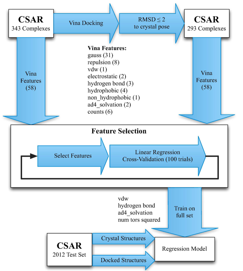
对接模式为刚性配体对接(rigid)或者柔性配体对接(flex),
刚性配体对接:配体自身保持刚性,经平移、旋转,在口袋内寻找合适的结合取向。
柔性配体对接:配体在固定某些非关键部位的键长、键角的前提下允许其构象发生一定程度的变化。
受体结构文件,PDB格式
配体结构文件,支持SDF、PDB、MOL格式。只会计算前2000的分子。
对接口袋中心的三维坐标(XYZ),空格分割。例如:0 0 0。
对接口袋长方体盒子的大小,必须是整数,空格分割,例如 24 22 32。
每个分子保留的最大结合模式数量
虚拟筛选中保留打分排名前n个分子。
保留非标准氨基酸,格式为[链名]:[残基名称]-[残基编号],如A:UNL-311。不能包含特殊离子的小分子结构。
输出结果包括:
| 输出文件名称 | 说明 |
|---|---|
| TopNScores.csv | 分子对接得到的打分csv文件。输出小分子最多为10,000。 |
| complex_001.pdb | 展示配体与受体的复合物构象文件。 |
| output_ligand_topn.sdf | 筛选后配体的SDF文件。根据指定的topN数生成,最多为10,000。 |
| output_complex_topn.tar.bz2 | 小分子与受体对接后的复合物构象PDB文件压缩包,最多生成前1000小分子的复合物结构。 |
Koes DR, Baumgartner MP, Camacho CJ. Lessons learned in empirical scoring with smina from the CSAR 2011 benchmarking exercise. J Chem Inf Model. 2013 Aug 26;53(8):1893-904.
Molecular Docking (SMINA) is a molecular docking tool based on SMINA. As a branch of Autodock Vina (http://vina.scripps.edu/), SMINA’s main function is to predict the binding modes and interactions between molecules, providing information on the energy and binding affinity of molecular docking. It can also calculate and compare the binding abilities of multiple molecules, useful for screening, designing, and optimizing drug molecules. Compared to Autodock Vina (version 1.1.2), SMINA supports:

Protein receptor structure file in PDB or PDBQT format. The receptor protein is set as rigid.
Small molecule structure file in SDF format.
Binding pocket information file in TXT format, obtainable from Weview. The file content is as follows:
center_x = -44.497
center_y = -22.273
center_z = -4.922
size_x = 40
size_y = 40
size_z = 40
Specify the top N small molecules for output, default is 100.
Number of conformations output for each ligand-protein docking, default is 10. This value should be ≤ “Run Pose”.
Define flexible residues in the format “chain name”:“amino acid number”, with each amino acid separated by a comma, e.g., “A:48,A:90,A:110”. Flexible amino acids must be near the pocket.
Set all side chains within a specified distance from the ligand as flexible, unit is Å.
Other parameters are the same as in Rigid Docking Mode.
The output includes:
| Output File Name | Description |
|---|---|
| Complex_Top1-10.pdb | Files showing the top ten complex conformations with the highest scores for each ligand-protein docking |
| score.csv | File containing scores for all ligand-protein dockings |
| TopNscore.csv | Scores file sorted by the highest docking scores for each ligand-protein docking |
| output.TopNComplex.tar.gz | Compressed file containing PDBQT files of the top complex conformations for each ligand-protein docking in the top N small molecules |
| output.TopNLigand.sdf | SDF file of the top N ligands based on docking scores |
Koes DR, Baumgartner MP, Camacho CJ. Lessons learned in empirical scoring with smina from the CSAR 2011 benchmarking exercise. J Chem Inf Model. 2013 Aug 26;53(8):1893-904.

Batch Renaming模块设计用于化学库的分子重命名。用户可以使用前缀和定义的长度来规范分子名称。例如,将一个从WCP0001开始的库重命名为WCP9999,用户可以输入WCP前缀,长度为4。用户还可以使用——keeptitle参数保存以前的名称,以保存名称之间的关系。该模块可用于大型从头库或用户私有化学库中的自定义分子命名。支持的输入文件格式为:SD(.sdf,.sd)。支持的输出文件格式为:SD(.sdf,.sd)。
小分子结构文件,SDF格式。
输出SDF文件名称。
自定义前缀,如C表示从C001生成名称,并结合长度为3。
固定名称长度,如4表示生成名C0001, 1表示生成C1, C2……。
新生成名称的位置:
字段名作为新生成的名称,仅当Location为filed或all时有效。
保留以前的分子标题名称。
得到重命名后的sdf文件output.sdf。
The Batch Renaming module is designed for renaming molecules in chemical libraries. Users can standardize molecule names using a prefix and a defined length. For example, to rename a library starting from WCP0001 to WCP9999, users can input the prefix WCP and a length of 4. Users can also use the --keeptitle parameter to preserve previous names, maintaining relationships between names. This module can be used for custom molecule naming in large de novo libraries or user-private chemical libraries. Supported input file formats: SD (.sdf, .sd). Supported output file formats: SD (.sdf, .sd).
Small molecule structure file in SDF format.
Name of the output SDF file.
Custom prefix, e.g., C indicating names generated from C001, combined with a length of 3.
Fixed name length, e.g., 4 generates names like C0001, 1 generates C1, C2, and so on.
Position for the newly generated names:
Field name to be used as the newly generated name, only valid when Location is field or all.
Keep the previous molecule title name.
Obtain the renamed SDF file named output.sdf.
3D Conf Generation (AlphaConf)采用唯信计算自研的分子三维构象生成算法,超快速生成分子三维构象库,比Open Eyes的Omega至少快一个数量级,后者被认为是目前最高效的商业产品。它也比薛定谔的ConfGenX快一个数量级以上。其优异的构象多样性和质量已被下游应用证明。AlphaConf非常适合用于药物分子发现的超高通量虚拟筛选。其技术特点如下:
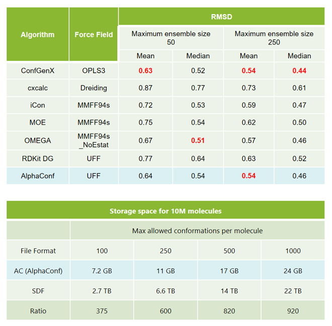
小分子结构文件,SDF格式或者压缩的SDF格式(.gz文件)。
每个分子的最大构象数,默认100。
构象能量截断值(单位:kcal/mol),默认20kcal/mol。
指定输出文件名称,后缀是.sd,.ac,.ac.gz或者.aux.gz。除了构象文件外,当输出文件后缀为.ac.gz或者.aux.gz还会输出片段库文件(文件后缀为.aux,其文件名根据构象文件名称自动命名,如:构象文件名设置为conf.ac.gz,片段文件名自动命名为conf.aux.gz)。
输出结果包括:
| 输出文件名称 | 说明 |
|---|---|
| SelfConf.ac.gz | 构象压缩文件,AC格式,用于AlphaShape模块的构象库输入 |
| SelfConf.aux.gz | 片段库文件(其文件名根据构象文件名称自动命名,如:构象文件名设置为conf.ac.gz或者conf.aux.gz,片段文件名自动命名为conf.aux),AUX格式,用于AlphaShape模块的片段库输入 |
3D Conf Generation (AlphaConf) uses a proprietary molecular conformation generation algorithm developed by Wecompute to rapidly generate a library of molecular conformations. It is at least an order of magnitude faster than Open Eye’s Omega, which is considered the most efficient commercial product, and more than an order of magnitude faster than Schrodinger’s ConfGenX. Its excellent conformational diversity and quality have been proven in downstream applications, making AlphaConf particularly suitable for high-throughput virtual screening in drug discovery. Its technical features are as follows:
Small molecule structure file in SDF format or gzip format with .gz file extension for SDF file.
The maximum number of conformations per molecule, the default value is 100.
Specify energy cutoff for confs.(kcal/mol), the default value is 20 kcal/mol.
Specify output conformation file in SD format(.sd) or AC format(.ac)
The output includes:
| Output File Name | Description |
|---|---|
| SelfConf.ac.gz | Conformation compressed file in AC format, used as input for the conformation library in the AlphaShape module. |
| SelfConf.aux.gz | Fragment library file in AUX format, used as input for the fragment library in the AlphaShape module. |

该模块可以去除或者统计分子含有的盐,从而获得去盐后分子结构或者分子结构含有的盐数量。
小分子结构文件,SDF或者SMILES格式。
输出文件名称。
选择去除(remove)或者统计(count)盐离子。
得到无盐离子的分子结构文件oufile.sdf。
The Salts Removal module can remove or count the salts present in molecules, providing the option to obtain the molecular structures without salts or the count of salts in the molecular structures.
Small molecule structure file in SDF or SMILES format.
Name of the output file.
Select whether to remove (remove) or count (count) salt ions.
Obtain a molecular structure file without salt ions named outfile.sdf.

基于规范SMILES字符串识别和删除重复分子,或者仅统计重复分子数量。支持的输入文件格式为:MOL(.mol)、SD(.sdf、.sd)、SMILES(.smi、.csv、.tsv、.txt)。支持的输出文件格式为:SD(.sdf、.sd)、SMILES(.smi、.csv、.tsv、.txt)。
小分子结构文件,SDF或者SMILES格式。
输出文件名称。
选择是去除重复分子(remove)还是对重复分子进行计数(count),默认为remove。
得到删除重复分子的sdf文件outfile.sdf。
The Duplicates Removal module identifies and removes duplicate molecules based on canonical SMILES strings, or it can simply count the number of duplicate molecules. Supported input file formats are: MOL (.mol), SD (.sdf, .sd), SMILES (.smi, .csv, .tsv, .txt). Supported output file formats are: SD (.sdf, .sd), SMILES (.smi, .csv, .tsv, .txt).
Small molecule structure file in SDF or SMILES format.
Name of the output file.
Select whether to remove duplicate molecules (remove) or count duplicate molecules (count), default is remove.
Obtain an SDF file named outfile.sdf after removing duplicate molecules.
基于多种2D指纹选择分子子集,使用MaxMin或可用的分层聚类方法,并将它们写入文件。RDKit中可用的Dice和Tanimoto相似性函数能够处理对应于IntVect和BitVect的指纹。然而,所有其他相似性函数都期望使用BitVect指纹来计算成对相似性。因此,对于AtomPairs、Morgan、MorganFeatures和TopologicalTorsions的相似性计算,使用ExplicitBitVect指纹代替默认的IntVect指纹。
小分子结构文件,SDF或者SMILES格式。
输出文件名称。
指定划分数量。
利用最大最小距离(MaxMin)或分层聚类方法(Hierarchical Clustering)进行聚类,从而选择不同的分子子集类型。
用于计算分子间相似性的方法,有Tanimoto、Cosine以及Dice。
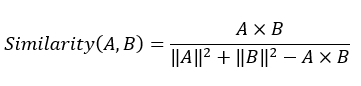
用于计算分子间相似性/距离的指纹。
按划分数量得到聚类结果,输出每个聚类中的第一个分子文件diverse_set.sdf。
The Diverse Subset module selects a subset of molecules based on multiple 2D fingerprints, using MaxMin or available hierarchical clustering methods, and writes them to a file. The Dice and Tanimoto similarity functions available in RDKit can handle fingerprints corresponding to IntVect and BitVect. However, all other similarity functions expect to use BitVect fingerprints to compute pairwise similarities. Therefore, for similarity calculations of AtomPairs, Morgan, MorganFeatures, and TopologicalTorsions, ExplicitBitVect fingerprints are used instead of the default IntVect fingerprints.
Small molecule structure file in SDF or SMILES format.
Name of the output file.
Specify the number of partitions.
Use MaxMin distance or hierarchical clustering to select different types of molecular subsets.
Methods used to calculate molecular similarity, including Tanimoto, Cosine, and Dice.
Fingerprints used to calculate molecular similarity/distance.
Cluster results are obtained based on the specified number of partitions, and the first molecule in each cluster is written to the file diverse_set.sdf.

Descriptors (RDKit)模块是计算分子的2D/3D描述符并将其写入SD或CSV/TSV文本文件中。2D描述符:Autocorr2D、MolWt、Ipc、NumRotatableBonds、qed等;3D描述符:Autocorr3D、RadiusOfGyration、Eccentricity等;以及FragmentCountOnly描述符:fr_Al_COO、fr_Al_OH、fr_Al_OH_noTert等。支持的输入文件格式为:Mol(.mol)、SD(.sdf、.sd)、SMILES(.smi、.txt、.csv、.tsv)。支持的输出文件格式为:SD文件(.sdf、.sd)、CSV/TSV(.csv、.tsv、.txt)。
小分子结构文件,SDF或者SMILES格式。
输出文件以保存计算的描述符。
使用多进程处理(默认:yes)。
计算分子描述符的类型,可选值有2D、3D、FragmentCountOnly和Specify。
2D描述符包括以下:
Autocorr2D, BalabanJ, BertzCT, Chi0, Chi1, Chi0n - Chi4n, Chi0v - Chi4v, EState_VSA1 - EState_VSA11, ExactMolWt, FpDensityMorgan1, FpDensityMorgan2, FpDensityMorgan3, FractionCSP3, HallKierAlpha, HeavyAtomCount, HeavyAtomMolWt, Ipc, Kappa1 - Kappa3, LabuteASA, MaxAbsEStateIndex, MaxAbsPartialCharge, MaxEStateIndex, MaxPartialCharge, MinAbsEStateIndex, MinAbsPartialCharge, MinEStateIndex, MinPartialCharge, MolLogP, MolMR, MolWt, NHOHCount, NOCount, NumAliphaticCarbocycles, NumAliphaticHeterocycles, NumAliphaticRings, NumAromaticCarbocycles, NumAromaticHeterocycles, NumAromaticRings, NumHAcceptors, NumHDonors, NumHeteroatoms, NumRadicalElectrons, NumRotatableBonds, NumSaturatedCarbocycles, NumSaturatedHeterocycles, NumSaturatedRings, NumValenceElectrons, PEOE_VSA1 - PEOE_VSA14, RingCount, SMR_VSA1 - SMR_VSA10, SlogP_VSA1 - SlogP_VSA12, TPSA, VSA_EState1 - VSA_EState10, qed
FragmentCountOnly描述符包括以下:
fr_Al_COO, fr_Al_OH, fr_Al_OH_noTert, fr_ArN, fr_Ar_COO, fr_Ar_N, fr_Ar_NH, fr_Ar_OH, fr_COO, fr_COO2, fr_C_O, fr_C_O_noCOO, fr_C_S, fr_HOCCN, fr_Imine, fr_NH0, fr_NH1, fr_NH2, fr_N_O, fr_Ndealkylation1, fr_Ndealkylation2, fr_Nhpyrrole, fr_SH, fr_aldehyde, fr_alkyl_carbamate, fr_alkyl_halide, fr_allylic_oxid, fr_amide, fr_amidine, fr_aniline, fr_aryl_methyl, fr_azide, fr_azo, fr_barbitur, fr_benzene, fr_benzodiazepine, fr_bicyclic, fr_diazo, fr_dihydropyridine, fr_epoxide, fr_ester, fr_ether, fr_furan, fr_guanido, fr_halogen, fr_hdrzine, fr_hdrzone, fr_imidazole, fr_imide, fr_isocyan, fr_isothiocyan, fr_ketone, fr_ketone_Topliss, fr_lactam, fr_lactone, fr_methoxy, fr_morpholine, fr_nitrile, fr_nitro, fr_nitro_arom, fr_nitro_arom_nonortho, fr_nitroso, fr_oxazole, fr_oxime, fr_para_hydroxylation, fr_phenol, fr_phenol_noOrthoHbond, fr_phos_acid, fr_phos_ester, fr_piperdine, fr_piperzine, fr_priamide, fr_prisulfonamd, fr_pyridine, fr_quatN, fr_sulfide, fr_sulfonamd, fr_sulfone, fr_term_acetylene, fr_tetrazole, fr_thiazole, fr_thiocyan, fr_thiophene, fr_unbrch_alkane, fr_urea
3D描述符包括以下:
Asphericity, Autocorr3D, Eccentricity, GETAWAY, InertialShapeFactor, MORSE, NPR1, NPR2, PMI1, PMI2, PMI3, RDF, RadiusOfGyration, SpherocityIndex, WHIM
此选项仅在Type为“Specify”时使用。当应用多个描述符时,由逗号分隔描述符,如MolWt, qed。
得到各个分子指定描述符的数值在descriptors.csv文件中。
The Descriptors (RDKit) module calculates 2D/3D descriptors of molecules and writes them to an SD or CSV/TSV text file. 2D descriptors include Autocorr2D, MolWt, Ipc, NumRotatableBonds, qed, etc.; 3D descriptors include Autocorr3D, RadiusOfGyration, Eccentricity, etc.; and FragmentCountOnly descriptors include fr_Al_COO, fr_Al_OH, fr_Al_OH_noTert, etc. Supported input file formats are: Mol (.mol), SD (.sdf, .sd), SMILES (.smi, .txt, .csv, .tsv). Supported output file formats are: SD files (.sdf, .sd), CSV/TSV (.csv, .tsv, .txt).
Small molecule structure file in SDF or SMILES format.
File to save the calculated descriptors.
Use multiprocessing for computation (default: yes).
Type of molecular descriptors to compute, options are 2D, 3D, FragmentCountOnly, and Specify.
2D descriptors include the following:
Autocorr2D, BalabanJ, BertzCT, Chi0, Chi1, Chi0n - Chi4n, Chi0v - Chi4v, EState_VSA1 - EState_VSA11, ExactMolWt, FpDensityMorgan1, FpDensityMorgan2, FpDensityMorgan3, FractionCSP3, HallKierAlpha, HeavyAtomCount, HeavyAtomMolWt, Ipc, Kappa1 - Kappa3, LabuteASA, MaxAbsEStateIndex, MaxAbsPartialCharge, MaxEStateIndex, MaxPartialCharge, MinAbsEStateIndex, MinAbsPartialCharge, MinEStateIndex, MinPartialCharge, MolLogP, MolMR, MolWt, NHOHCount, NOCount, NumAliphaticCarbocycles, NumAliphaticHeterocycles, NumAliphaticRings, NumAromaticCarbocycles, NumAromaticHeterocycles, NumAromaticRings, NumHAcceptors, NumHDonors, NumHeteroatoms, NumRadicalElectrons, NumRotatableBonds, NumSaturatedCarbocycles, NumSaturatedHeterocycles, NumSaturatedRings, NumValenceElectrons, PEOE_VSA1 - PEOE_VSA14, RingCount, SMR_VSA1 - SMR_VSA10, SlogP_VSA1 - SlogP_VSA12, TPSA, VSA_EState1 - VSA_EState10, qed
FragmentCountOnly descriptors include the following:
fr_Al_COO, fr_Al_OH, fr_Al_OH_noTert, fr_ArN, fr_Ar_COO, fr_Ar_N, fr_Ar_NH, fr_Ar_OH, fr_COO, fr_COO2, fr_C_O, fr_C_O_noCOO, fr_C_S, fr_HOCCN, fr_Imine, fr_NH0, fr_NH1, fr_NH2, fr_N_O, fr_Ndealkylation1, fr_Ndealkylation2, fr_Nhpyrrole, fr_SH, fr_aldehyde, fr_alkyl_carbamate, fr_alkyl_halide, fr_allylic_oxid, fr_amide, fr_amidine, fr_aniline, fr_aryl_methyl, fr_azide, fr_azo, fr_barbitur, fr_benzene, fr_benzodiazepine, fr_bicyclic, fr_diazo, fr_dihydropyridine, fr_epoxide, fr_ester, fr_ether, fr_furan, fr_guanido, fr_halogen, fr_hdrzine, fr_hdrzone, fr_imidazole, fr_imide, fr_isocyan, fr_isothiocyan, fr_ketone, fr_ketone_Topliss, fr_lactam, fr_lactone, fr_methoxy, fr_morpholine, fr_nitrile, fr_nitro, fr_nitro_arom, fr_nitro_arom_nonortho, fr_nitroso, fr_oxazole, fr_oxime, fr_para_hydroxylation, fr_phenol, fr_phenol_noOrthoHbond, fr_phos_acid, fr_phos_ester, fr_piperdine, fr_piperzine, fr_priamide, fr_prisulfonamd, fr_pyridine, fr_quatN, fr_sulfide, fr_sulfonamd, fr_sulfone, fr_term_acetylene, fr_tetrazole, fr_thiazole, fr_thiocyan, fr_thiophene, fr_unbrch_alkane, fr_urea
3D descriptors include the following:
Asphericity, Autocorr3D, Eccentricity, GETAWAY, InertialShapeFactor, MORSE, NPR1, NPR2, PMI1, PMI2, PMI3, RDF, RadiusOfGyration, SpherocityIndex, WHIM
This option is only used when Type is “Specify.” When applying multiple descriptors, separate them by commas, e.g., MolWt, qed.
The numerical values of the specified descriptors for each molecule are stored in the descriptors.csv file.

PAINS Filter模块通过SMARTS子结构规则来搜索输入文件中假阳性化合物(Pan-assay Interference molecules,PAINS),并将符合条件的分子输出或者统计过滤分子的数量。
小分子结构文件,SDF或者SMILES格式。
输出文件名称。
是否使用多进程进行计算,可选:yes或者no,默认为yes。
输出文件包含与PAINS匹配的分子,可选:yes或者no,默认为no。
输出结果包括:
| 输出文件名称 | 说明 |
|---|---|
| output.sdf | 筛选出不匹配PAINS规则的化合物 |
| output_Filtered.sdf | 筛选出匹配PAINS规则的化合物 |
The PAINS Filter module searches for false positive compounds (Pan-assay Interference molecules, PAINS) in the input file using SMARTS substructure rules and either outputs or counts the molecules that meet the criteria.
Small molecule structure file in SDF or SMILES format.
Name of the output file.
Whether to use multiprocessing for computation, options: yes or no, default is yes.
Whether the output file includes molecules that match PAINS, options: yes or no, default is no.
The output includes:
| Output File Name | Description |
|---|---|
| output.sdf | Compounds that do not match the PAINS rules |
| output_Filtered.sdf | Compounds that match the PAINS rules |

File是用于指定输入文件的模块,可用于多个模块的统一输入。
上传小分子结构文件(SDF格式)或者蛋白的结构文件(PDB格式)
输出重命名后的文件。
The File module is used to specify input files and can be used for unified input across multiple modules.
Upload a small molecule structure file (SDF format) or a protein structure file (PDB format).
Output the file after renaming.
PDB文件是一个用于指定PDB文件的模块,可用于其他模块的输入。
Protein structure file in PDB format
得到PDB文件
The PDB File module is used to specify a PDB file that can be used as input for other modules.
Protein structure file in PDB format.
Obtain a PDB file.